
4.3 Permanent Magnet Systems: Design and Analysis
Understanding Permanent Magnet Systems
Permanent-magnet systems are integral to many modern technologies, enabling the generation of a steady magnetic field without the need for external power. These systems rely on permanent magnets, which are materials capable of retaining their magnetic properties over time.Permanent magnets are widely used in electric motors, generators, magnetic separators, medical imaging devices, and various other applications. Let's explore their key features, behavior, and relevant formulas to understand how they work.
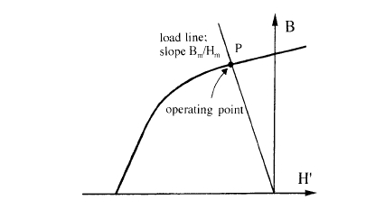
Figure 4.22. Demagnetizing characteristic for a permanent magnet, showing the load line and the working point.
because \(H\) is oppositely directed within the magnet and outside it. Magnetic flux \(\Phi\) (analogous to electric current) flows out of the magnet and around the circuit, since flux, like dc current in a circuit with no capacitance, has no divergence. Each component in the circuit has a permeance (analogous to conductance) defined as \(\Phi/\psi_{\mathrm{m}}\), which is a product of the permeability and the dimensions of the element, \(\mu_0\) is the permeability of free space. If a component had infinite permeance, there would be no drop in magnetostatic potential \(\psi_{\mathrm{m}}\) across it and no field within it. The permeance \(P_{\mathrm{g}}\) of a short air - gap of cross - sectional area \(A_{\mathrm{g}}\) and length \(l_{\mathrm{g}}\) is given by \(P_{\mathrm{g}}=\Phi_{\mathrm{g}}/\psi_{\mathrm{g}} = B_{\mathrm{g}}A_{\mathrm{g}}/H_{\mathrm{g}}l_{\mathrm{g}} = \mu_0A_{\mathrm{g}}/l_{\mathrm{g}}\). The magnet itself has a permeance (analogous to the internal conductance of a battery) which depends on the shape and magnetization of the magnet, that determines \(B\) and \(H'\) within it: \(P_{\mathrm{m}} = B_{\mathrm{m}}A_{\mathrm{m}}/H_{\mathrm{m}}l_{\mathrm{m}}\). The ratio \(B_{\mathrm{m}}/H_{\mathrm{m}}\) in zero external field is the slope of the load line (figure 4.22). The permeance of circuit components in parallel, such as flux is divided, add directly, whereas circuit components in series such as pole pieces and the main air - gap contain the same flux and the inverse permeance \(R\), known as reluctance (analogous to electrical resistance), adds figure 4.23. A simple magnetic circuit and its electrical equivalents are shown.
Magnetic circuit design is a process that requires experience on the part of the engineer because of the flux leakage around every component. A typical procedure is to make a model circuit with the aid of a toolkit of standard permeances and then build a real magnetic circuit and measure its characteristics, such as the potential \(\varphi_{\mathrm{m}}\) at points around it, the flux density \(B\) and field \(H'\) in the magnet and \(H\) in air at helpful points. After improving the design based on this information, it may be helpful to model the circuit in two or three dimensions on a workstation. Numerical design strategies based on optimization procedures,
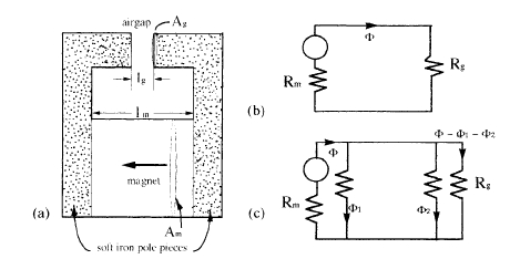
Figure 4.23. (a) A simple magnetic circuit composed of a magnet, soft-iron segments and an airgap. with equivalent electric circuits, ( b) assuming there are no flux losses in the iron or the gap and (c) allowing for the flux losses. such as simulated annealing, are also beginning to be employed. However, it should be emphasized that the result of any numerical study can only be as good as the accuracy of the description of materials’ properties which are provided as input.
System Measurements: Techniques for Evaluating Permanent Magnets
Measurements of permanent magnets, as opposed to specimens of magnetic material, involve no externally applied magnetic field unless one is produced by excitation coils in a device such as a motor. Properties of interest include the magnetic moment of the magnet \(m\), the scalar potential \(\varphi_{\mathrm{m}}\) and the fields \(H\) and \(B\) inside the magnet which define the load line and the working point (figure 4.22).
The magnetic moment can be measured by one of the methods described in the previous section. No external field is required. The magnet may be removed from the centre of a search coil or vibrated at the centre of an oppositely wound Helmholtz pair. In either case, an induced emf proportional to the magnetic moment is measured. Calibration involves using a similarly shaped magnet of known \(m\) in the same conditions. The magnetization \(M\) is then \(m/V\), where \(V\) is the magnet volume.
The flux density \(B\) produced in a magnet of uniform cross - section \(A\) can be determined by winding a close - fitting coil around it which is connected to a fluxmeter. The flux change is registered as the magnet is slipped out of the coil and taken away. Whenever this is impractical because of the magnet shape or because it is built into a larger structure, the \(H\) field may be deduced from the
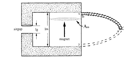
Figure 4.24. Use of a potential coil to measure magnetic potential difference between two points of a magnetic circuit.
magnetostatic potential \(\varphi\) measured using the potential coil of cross - section \(A_{\mathrm{c}}\) having \(n\) turns per metre (figure 4.23). Keeping one end 'a' fixed and moving the other end 'b' from point \(x\) to point \(y\) on a magnetic circuit generates a change of flux \(\Delta\Phi=-\mu_{0}nA_{\mathrm{c}}(\varphi_{x}-\varphi_{y})\). This flux change is registered directly by the fluxmeter, hence the potential difference \(\varphi_{x - y}=(\varphi_{x}-\varphi_{y})\) is deduced from the constants of the potential coil (figure 4.24). Assuming \(H\) is uniform in a magnet of length \(l\), \(H=\varphi_{x - y}/l\). Likewise, measurement of \(\varphi\) between other points of the circuit gives an idea of \(H\) in each circuit element, which may be related to flux leakage. Alternatively, a Hall probe may be placed close beside the circuit element to read the field component \(H_{\parallel}\) parallel to the surface, which is continuous.
Computer Modeling and Field Calculations: Simulating Magnetic Systems
In principle, any problem in electromagnetism can be modelled by solving Maxwell's equations numerically at a sufficient number of points in space, with appropriate boundary conditions. The equations can be considered in their integral form (\(\oint\boldsymbol{B}\cdot\mathrm{d}\boldsymbol{S}=0\)) or in their differential form (\(\nabla\cdot\boldsymbol{B}=0\) etc.). The fields \(\boldsymbol{B}\) and \(\boldsymbol{H}\) can be deduced from the potentials \(A\) and \(\varphi_{\mathrm{m}}\), when appropriate. The reason for using potentials rather than fields is that difficulties arising from field discontinuities at material boundaries can be avoided. The problem then becomes one of numerical solution of second - order differential equations.
A purely magnetostatic problem is described by the simplified Maxwell equations (1.6) and (2.5)
\(\nabla\cdot\boldsymbol{B}=0\) and \(\nabla\times\boldsymbol{H}' = 0\) (4.16)
plus the equation of state of the magnetic material,
\(\boldsymbol{B}=\boldsymbol{B}(\boldsymbol{H}')\) or \(M = M(H')\) (4.17)
where \(B=\mu_{0}(H'+M)\). Note that any two of the three quantities \(B\), \(H'\) and \(M\) serve to define the system. The equation of state is generally nonlinear and is not single valued. In a paramagnet or soft ferromagnet it is single valued and may be written as \(M=\chi H'\), where the susceptibility is constant for an isotropic material far from saturation. Otherwise \(\chi\) is a tensor and a function of \(H'\). A hard magnet in its operating range can be approximately represented by
\(M_{\parallel}=\chi_{\parallel}H_{\parallel}+M_{\mathrm{r}}\) (4.18a)
\(M_{\perp}=\chi_{\perp}H_{\perp}\) (4.18b)
where \(\chi_{\parallel}\) is the parallel susceptibility at remanence, \(\chi_{\perp}\) is the transverse susceptibility and \(M_{\mathrm{r}}\) is the remnant magnetization. An ideal permanent magnet would have \(M_{\mathrm{r}} = M_{\mathrm{s}}\), \(\chi_{\parallel}=0\) and \(\chi_{\perp}=\mu_{0}M_{\mathrm{s}}^{2}/2K_{1}\). Often \(\chi_{\perp}\) is neglected, but a glance at the ratio \(M_{\mathrm{r}}/H_{0}\) in table 3.8 shows that this is only really justified for \(\text{SmCo}_{5}\).
Provided no conduction currents are involved, it is possible to define \(H'\) in a straightforward way as the gradient of the scalar potential \(\varphi\) which is single valued at every point. \(H'=-\nabla\varphi_{\mathrm{m}}\). This follows since the curl grad operation \(\nabla\times\nabla\) is identically zero. Taking the divergence of \(\nabla\varphi_{\mathrm{m}}=-H'\) yields Poisson's equation (2.6)
\(\nabla^{2}\varphi_{\mathrm{m}}=\nabla\cdot M\) (4.19)
where div grad has been written as \(\nabla^{2}\) and \(-\nabla\cdot H'\) is equal to \(\nabla\cdot M\), since \(\boldsymbol{B}=\mu_{0}(H'+M)\) and \(\nabla\cdot\boldsymbol{B}=0\). The quantity \(\nabla\cdot M\) is zero outside a magnet, where \(M\) is zero, and it is also zero inside whenever \(M\) is uniform. Equation (4.19) then reduces to Laplace's equation \(\nabla^{2}\varphi_{\mathrm{m}} = 0\). It is only at the surfaces of a uniformly magnetized block that \(\nabla\cdot M\neq0\). There it is possible to imagine a sheet of surface charge \(\sigma_{\mathrm{m}}=M\cdot\boldsymbol{e}_{\mathrm{n}}\), where \(\boldsymbol{e}_{\mathrm{n}}\) is the outward normal at the surface which acts as the source of \(H\). The normal component of \(H\) changes by \(\sigma_{\mathrm{m}}\) on crossing the surface. The potential \(d\varphi_{\mathrm{m}}\) and field \(dH\) due to a small charge element \(d q_{\mathrm{m}}=\sigma_{\mathrm{m}}dS\) are
\(d\varphi_{\mathrm{m}}=d q_{\mathrm{m}}/4\pi r\) (4.20)
and
\(dH = d q_{\mathrm{m}}\boldsymbol{e}_{\mathrm{n}}/4\pi r^{2}\) (4.21)
This scalar potential approach is most useful for calculating the fields and forces between magnets represented by sheets of surface charge. In simple cases, results can be found analytically. Otherwise they may be deduced by numerical integration over a surface, a procedure known as the boundary element method.
A more general magnetic situation arises in electrical devices where there are conductors carrying steady or slowly varying currents. The displacement
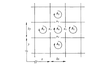
Figure 4.25. A grid used to obtain numerical solutions of differential equations in two dimensions using the finite - difference method.
The remanence can be assimilated as an effective current \(\boldsymbol{j}_{\mathrm{r}}\). The second - order differential equation for \(\boldsymbol{A}\) becomes
\(\nabla\times\nu\nabla\times\boldsymbol{A}=\mu_{0}(\boldsymbol{j}+\boldsymbol{j}_{\mathrm{r}})\) (4.26)
where the reluctivity \(\nu = 1/\mu\). In a two - dimensional problem only the components \(A_{z}\) and \(\nu\) generate fields in the \(x - y\) plane, and \(B_{x}=\partial A_{z}/\partial y\), \(B_{y}=-\partial A_{z}/\partial x\). The equation for \(A_{z}\) becomes
\(\frac{\partial(\nu\partial A_{z}/\partial x)}{\partial x}+\frac{\partial(\nu\partial A_{z}/\partial y)}{\partial y}=-\mu_{0}j_{z}\) (4.27)
For a numerical solution, the partial derivatives are expressed as difference approximations. An array of points is set up in the \(x - y\) plane where values of \(A\) and \(\nu\) are defined, as illustrated in figure 4.25. If the separation of the points is \(\delta_{x}=\delta_{y}=\delta\), then, for example,
\(\frac{\nu_{1}(A_{1}-A_{0})/\delta-\nu_{3}(A_{0}-A_{3})/\delta+\nu_{2}(A_{2}-A_{0})/\delta-\nu_{4}(A_{0}-A_{4})/\delta}{\delta}=-\mu_{0}j_{z}\) (4.28)
Hence \(A_{0}=[\sum\nu_{i}A_{i}+\delta^{2}\mu_{0}j_{z}]/\sum\nu_{i}\) and similarly for all the other cells. Taking a plausible set of \(A_{i}\)s to begin with, the \(A_{i}\) values are refined by repeated scanning over all the points on the network. Then \(B\) is calculated at any point in the plane as curl \(\boldsymbol{A}\). The finite - difference method is slow, but there are special numerical techniques which will accelerate convergence.
An alternative approach involves the scalar potential \(\varphi_{\mathrm{m}}\). Instead of taking the curl of \(\boldsymbol{B}=\mu_{0}(\mu\boldsymbol{H}'+\boldsymbol{M}_{\mathrm{r}})\) as in (4.25), we operate with div, yielding
\(\nabla\cdot\mu\nabla\varphi_{\mathrm{m}}+\nabla\cdot\boldsymbol{M}_{\mathrm{r}} = 0\) (4.29)
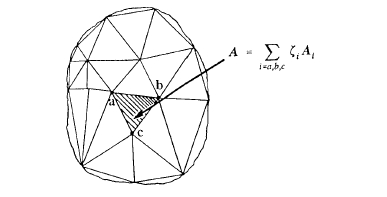
Figure 4.26. Triangular mesh used for a two - dimensional finite - element calculation.
This differential equation can likewise be solved by the finite - difference method to give \(\varphi_{\mathrm{m}}\). If \(\boldsymbol{M}_{\mathrm{r}}\) is uniform there is only a contribution from surface charges, as discussed in (4.20).
The finite - element method is increasingly used to model electromagnetic devices. Space occupied by and surrounding the device is tessellated by a suitably adapted triangular mesh for the two - dimensional problem and by a tetrahedral mesh for the three - dimensional problem. Within each element, the potential is described by its nodal values with appropriate weighting functions \(\zeta_{i}\). Taking the scalar potential in two dimensions for example,
\(\varphi_{\mathrm{m}}=\sum\zeta_{i}\varphi_{i}\) (4.30)
Next, an energy functional \(F\) is defined which is an integral over \(\Omega\), the whole space of interest. The functional for the two - dimensional problem involving scalar potential would be
\(F=\int f(x,y,\varphi_{\mathrm{m}},\partial\varphi_{\mathrm{m}}/\partial x,\partial\varphi_{\mathrm{m}}/\partial y)d\Omega_{\varphi_{\mathrm{m}}}\) (4.31)
This integral is minimized when the Euler equations are satisfied:
\(\partial f/\partial\varphi_{\mathrm{m}}-d/dx(\partial f/\partial\varphi_{\mathrm{m}}') = 0\) (4.32)
\(F\) is chosen so that these coincide with the differential equations which should be satisfied by the potential. For example, the functional which yields (4.30) is
\(F=-\int[\varphi_{\mathrm{m}}\cdot\nabla\cdot\mu\nabla\varphi_{\mathrm{m}}-2\varphi_{\mathrm{m}}\cdot\nabla\cdot\boldsymbol{M}_{\mathrm{r}}]d\Omega_{\varphi_{\mathrm{m}}}\) (4.33)
The energy functional is evaluated for each element in terms of the nodal potentials by substituting (4.30) into (4.33), and the functional is minimized by setting \(dF/d\varphi_{i}=0\) for each element which gives a set of equations describing the entire problem. This provides the potential distribution. Like finite - difference method, the procedure is iterative and it continues until the residuals are acceptably small. The required fields are obtained in the post - processing stage.
Finite - element software packages are available to model magnetic systems in two and three dimensions. Adaptive meshes can be generated automatically and the packages are a valuable design tool for the magnetic engineer.


