

3.4 Magnetic Viscosity: Understanding Time-Dependent Magnetism
The non-equilibrium character of permanent magnetism means that thermal excitations drive the magnetization \(M(\mathbf{r})\) towards equilibrium. The associated time dependence of extrinsic magnetic properties such as remanence and coercivity is known as magnetic viscosity, magnetic after-effect or ageing. A simplistic but very instructive approach is to write the relaxation time as an exponential Arrhenius decay \(\tau/\tau_{0}=\exp(K_{1}V_{0}/k_{\text{B}}T)\). Taking \(\tau_{0}=10^{-9}\ s^{28}\), \(K_{1}=1\ MJ\ m^{-3}\) and a room-temperature 'life expectancy' of about 1000 years yields the activation volume \(V_{0}\approx 200\ nm^{3}\). This means that laboratory-scale magnetic viscosity involves regions whose radii are smaller than about 3.6 nm. It is worth noting that \(K_{1}V_{0}/k_{\text{B}}\) defines a fictitious activation temperature much larger than room temperature.
Experiment shows that the time-dependence of the magnetization is reasonably well described by the logarithmic law
\(M(t,H)=M(t_{0},H)-S(H)\ln\frac{t}{t_{0}}\). (3.118)
Here \(S\) is a phenomenological magnetic viscosity constant and \(t_{0}\) is a reference time. \(S\) and \(\mu_{0}S\) are measured in \(A\ m^{-1}\) and \(T\), respectively. The logarithmic law, whose origin will be explained in section 3.4.2, means that
the magnetization decay is rather strong in the short term but remains largely unaltered in the medium and long term.
From the point of view of atomic physics, magnetic viscosity is a macroscopic relaxation phenomenon. A simple description of relaxation phenomena is given by the Landau–Lifshitz equation
\(\frac{\text{d}\mathbf{M}}{\text{d}t} = \gamma_{0}\mathbf{M} \times \mathbf{H}_{\text{eff}} - \frac{1}{M_{\text{s}}^{2}\tau_{0}}\mathbf{M} \times (\mathbf{M} \times \mathbf{H}_{\text{eff}})\) (3.119)
where \(\gamma_{0} = g\mu_{\text{B}}/\hbar\) is the gyromagnetic ratio, \(\tau_{0}\) denotes a microscopic relaxation term and \(\mathbf{H}_{\text{eff}} = -\delta E(\mathbf{M})/\delta(\mu_{0}\mathbf{M})\) is the effective field acting on the magnetization. Aside from the precession of the magnetization, (3.119) describes the viscous rotation of \(\mathbf{M}\) towards \(\mathbf{H}_{\text{eff}}\), that is relaxation in the vicinity of local or global energy minima. However, the Landau–Lifshitz equation, and similar relations such as the Gilbert and Bloch–Bloembergen equations, are unable to explain thermally activated transitions (jumps) over barriers separating metastable or global energy minima.
Non-Equilibrium Statistical Mechanics: The Foundation of Magnetic Viscosity
This subsection is devoted to the non-equilibrium statistical mechanics of permanent magnets. Since the number of exact quantum-statistical solutions is very limited, we will first consider a number of simple models. Magnetic viscosity in real permanent magnets is dealt with in section 3.4.3.
Atomic Spin Dynamics
To discuss the evolution of a quantum-mechanical system, one has to consider the time-dependent Schrödinger equation
\(i\hbar\frac{\partial}{\partial t}|\Psi\rangle = \mathcal{H}|\Psi\rangle\) (3.120)
or, alternatively, the Liouville–von Neumann equation
\(i\hbar\frac{\text{d}\hat{\rho}}{\text{d}t} = \mathcal{H}\hat{\rho} - \hat{\rho}\mathcal{H}\) (3.121)
where \(\hat{\rho} = |\Psi(t)\rangle\langle\Psi(t)|\) is the density operator. Note that thermal averages are easily calculated from \(\hat{\rho}(t)\)
\(\langle A(t)\rangle = \text{Tr}(\hat{A}(t)\hat{\rho}(t))\) (3.122)
where \(\hat{A}\) is any quantum-statistical observable.
According to (3.120), the behaviour of isolated atomic spins in an external field \(\mathbf{H} = H\mathbf{e}_{z}\) is determined by the equation
\(i\hbar\frac{\partial\psi}{\partial t} = -\mu_{0}\mu_{\text{B}}H\hat{\sigma}_{z}\psi\) (3.123)
where the spin matrix \(\hat{\sigma}_{z}\), introduced in equation (2.17), describes the Zeeman interaction with the external field. The solution of this equation is the two-component wavefunction
\(\psi(t) = (\psi_{1}\text{e}^{i\omega t}, \psi_{2}\text{e}^{-i\omega t})\) (3.124)
where the paramagnetic resonance frequency \(\omega = \mu_{0}\mu_{\text{B}}H/\hbar\) is in the GHz region for fields of the order of 1 T.
Fixing the wavefunction of (3.123) by the initial condition \(\psi(0) = (1/\sqrt{2})(1, 1)\) yields \(\langle\sigma_{x}(t)\rangle = \cos(2\omega t)\) and \(\langle\sigma_{z}(t)\rangle = 0\). This means that a field in the \(z\)-direction causes the spin components in the \(x - y\) plane to precess around the \(z\)-axis. On the other hand, putting \(\psi(0) = (0, 1)\), yields \(\langle\sigma_{z}(t)\rangle = -1\) and \(\langle\sigma_{x}(t)\rangle = 0\). This means that a magnetic field in the \(z\)-direction is unable to change the spin projection in the \(z\)-direction. Equation (3.121) cannot therefore explain why magnetic reversal occurs in a magnetic field antiparallel to the magnetization. Furthermore, there is no temperature dependence in (3.121).
Relaxation
Ultimately, magnetic reversal is caused by the interaction of the magnetic moments with other degrees of freedom such as lattice vibrations. Equation (3.120) can be used to predict the evolution of any physical system, but this method is not feasible in practice. For example, exploiting the fact that the entropy operator \(\hat{S} = -k_{\text{B}}\ln\hat{\rho}\) commutes with \(\hat{\rho}\) one finds that \(dS/dt = 0\).
This counterintuitive result reflects the deterministic character of the exact Schrödinger and Liouville–von Neumann equations. Since the eigenenergy spectrum of a Hamiltonian describing a large but finite system is discrete, typical level spacings \(\Delta E\) give rise to a finite though possibly very large recurrence time \(t \approx \hbar/\Delta E\). In the thermodynamic limit of an infinite number of degrees of freedom, the recurrence time goes to infinity and the dynamics of the system become irreversible.
In practice, one does not consider truly large systems but transforms the complete Hamiltonian \(\mathcal{H}\) into a 'coarse-grained' Hamiltonian. The coarse-grained Hamiltonian describes the interesting relevant magnetic degrees of freedom, whereas irrelevant magnetic and non-magnetic degrees of freedom, such as phonons and magnons, are considered as a heat bath. The heat bath can also be interpreted in terms of random thermal forces acting on the local magnetization, because the heat-bath fluctuations are much faster than the magnetization changes in question. On an atomic scale, the thermal forces ensure equilibrium and realize, for example, the spontaneous magnetization \(M_{\text{s}}(T)\). In this sense it is meaningful to regard the magnetic energy as an equilibrium free energy. On the other hand, the relaxation of the relevant degrees of freedom, such as the average magnetization of a crystallite, is much slower and cannot be described by equilibrium statistics.
Non-Equilibrium and The Master Equation
It is possible but very cumbersome to derive explicit equations of motion from the coarse-grained Liouville–von Neumann equations. Here we use a different approach: we construct a non-equilibrium equation of motion and show how this equation relates to (3.120) and (3.121). For simplicity, we will restrict ourselves to a single relevant degree of freedom \(s\). Examples are \(s = \sin\theta\) in fine-particles and \(s\) being proportional to the well displacement in pinning-type magnets.
Consider the energy landscape \(E(s)\) shown in figure 3.39. Typically, the height of the energy barrier, \(E_{0}\), is proportional to \(K_{1}\). In equilibrium, the symmetry of the potential \(E(s)\) implies zero magnetization: \(\langle s\rangle = 0\). To explain remanence and magnetic viscosity we apply a strong external magnetic field. Switching off the field at \(t = 0\) then yields the initial spin distribution shown in figure 3.39, where \(\langle s\rangle = 1\). Note that the point distribution shown in figure 3.39 is an ensemble average, that is a large number of experiments monitored at \(t = 0\). By contrast, time averaging amounts to making a series of snapshots at different times29. The problem is now to describe the evolution of the ensemble probability distribution \(P(s)\).
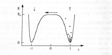
Figure 3.39. A model potential illustrating the process of magnetic viscosity. Each arrow shows the net probability flux.
A conceptually simple approach is the introduction of transition rates \(W(s, s')\) describing transitions from \(s'\) to \(s\). This leads to the master equation
\(\frac{\partial P(s)}{\partial t} = \int[W(s, s')P(s') - W(s', s)P(s)]\text{d}s'\) (3.125)
where the second term on the right-hand side ensures the time independence of the normalization \(\int P(s)\text{d}s = 1\). In equilibrium \(\partial P / \partial t = 0\) and \(P(s) \propto \exp(-V(s)/k_{\text{B}}T)\), which is realized by the detailed balance condition
\(W(s, s') = \exp\left(\frac{E_{\text{m}}(s') - E_{\text{m}}(s)}{k_{\text{B}}T}\right)W(s, s')\). (3.126)
Master equations based on calculated or phenomenological transition rates are a widely used tool in non-equilibrium statistics. For example, the Glauber model describing the dynamics of the Ising model is based on \(W(-s, s) \propto (1 - s\tanh(h/k_{\text{B}}T))\), where \(h\) is an interaction field. A master equation will be used in section 3.4.3.4.3.
The Langevin and Fokker–Planck Equations
An atomic approach towards magnetic viscosity is to consider random thermal forces \(\xi(t)\) acting on the magnetization vector. This leads to the Langevin equation
\(\frac{\partial s}{\partial t} = -\frac{\Gamma_{0}}{k_{\text{B}}T}\frac{\partial E}{\partial s} + \sqrt{2\Gamma_{0}}\xi(t)\) (3.127)
where \(\Gamma_{0} = 1/\tau_{0}\) is an atomic attempt frequency. The random forces obey
\(\langle\xi(t)\xi(t')\rangle = \delta(t - t')\)
\(\langle\xi(t)\rangle = 0\)
where \(\delta(x)\) is the delta function defined by \(\delta(x) = 0\) for \(x \neq 0\) and \(\int\delta(x)\text{d}x = 1\). The \(\partial E / \partial s\) term in (3.127) corresponds to the last term in (3.119), but in contrast to (3.119) and (3.123) there is no precession term in this equation, because the atomic precession period is much smaller than the macroscopic equilibration time under consideration. On the other hand, the random-force term in (3.127) makes it possible to overcome energy barriers. Note that the coarse-graining procedure mentioned in section 3.4.1.2 leads to a modified Liouville–von Neumann equation, where the coupling to the heat bath is reflected by relaxation and random-force terms equivalent to the respective \(\partial s / \partial t\) and \(\xi\) terms in (3.127).
At low temperatures, the \(\partial s / \partial t\) and \(\xi\) terms are negligible and (3.127) reduces to the trivial minimization problem \(\partial E / \partial s = 0\). At finite temperatures, it can be solved by calculating \(s(t)\) for a large number of random functions \(\xi(t)\). However, in practice it is often sufficient to know the probability distribution \(P(s, t)\). This probability distribution obeys the magnetic Fokker–Planck equation
\(\tau_{0}\frac{\partial P}{\partial t} = \frac{1}{k_{\text{B}}T}\frac{\partial}{\partial s}\left(P\frac{\partial E}{\partial s}\right) + \frac{\partial^{2}P}{\partial s^{2}}\). (3.129)
An alternative way of deriving (3.129) is the Kramers–Moyal expansion of the transition rates \(W(s, s')\) into powers of the small quantity \(s - s'\). Physically, the
Langevin and Fokker–Planck equations imply that macroscopic magnetization jumps consist of a chain of microscopic events. They neglect, for example, the extremely unlikely event that the thermally activated motion of a single atom leads to magnetic reversal. Note that the Fokker–Planck equation can be interpreted as a generalized diffusion equation. In equilibrium (\(\partial P / \partial t = 0\)), it reproduces the Boltzmann distribution \(P(s) = (1/Z)\exp(-E/k_{\text{B}}T)\).
Linear Viscosity
It is instructive to compare magnetic hysteresis with linear viscosity. Putting the energy \(E(s) = E_{0}(s^{2}/2 - \chi_{0}Hs/M_{\text{s}})\) into (3.127) yields the averaged equation of motion
\(\tau_{\text{eff}}\frac{\text{d}M}{\text{d}t} = -M + \chi_{0}H\) (3.130)
where \(M = \langle s\rangle M_{\text{s}}\) and \(\tau_{\text{eff}} = k_{\text{B}}T / \Gamma_{0}E_{0}\). This equation assimilates magnetic viscosity to a linear viscous medium. It is easy to show that an applied field \(H = H_{0}\sin(\omega t)\) yields \(M = M_{0}\sin(\omega t - \phi)\), where \(\tan(\phi) = \omega\tau\). On the other hand, by setting \(M = 0\) in (3.130) we see that the \(\text{d}M/\text{d}t\) term gives rise to an \(\omega\)-dependent coercivity. The explicit coercivity expression \(H_{\text{c}} = H_{0}\omega\tau/(1 + \omega\tau)\) illustrates the fact that \(H_{\text{c}} = 0\) in the equilibrium limit \(\omega = 0\).
However, magnetic hysteresis is not only a non-equilibrium but also a nonlinear problem. This is seen, for example, from the equilibrium magnetization \(M = \chi_{0}H\) derived from (3.130), which leads to an unphysical divergence of \(M\) in the limit of very high fields. The reason is that (3.130) is obtained from the Langevin equation (3.127) by using an energy expression quadratic in \(s = M/M_{\text{s}}\). In fact, to assure a finite magnetization in infinite fields one needs bistable (at least quartic) potentials such as that shown in figure 3.39.
The Logarithmic Law: A Key Principle in Magnetic Viscosity
Equation (3.118) means the decay of some percentage of the magnetization per decade. For example, if there is a remanence loss of 0.5% between one day and ten days after production (magnetizing) then there will be another 0.5% of loss between the 10th and 100th days. Figure 3.40 compares the logarithmic and exponential decay laws. The magnetic viscosity \(S\) is an extrinsic property and therefore strongly morphology dependent. Magnetic viscosity is largest in the vicinity of \(H_{\text{c}}\), where the energy barrier is lowest. A typical room-temperature value is \(\mu_{0}S(H_{\text{c}}) = 36\ mT\) for sintered Nd2Fe14B, so that the magnetization loss is of the order of 80 \(mT\) per decade.
Basic Features
A simple derivation of the logarithmic law relies on the assumption of an ensemble of independent relaxation processes where the relaxation time of the
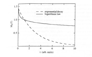
Figure 3.40. Magnetic viscosity (schematic).
i th relaxer is\(\tau_{\mathrm{r}}=\tau_{0} \exp \left(E_{\mathrm{f}} / k_{\mathrm{B}} T\right)^{30}\). In a reverse field, the relaxations give rise to the time dependence
\(M(t)=-M_{\mathrm{s}}+2 M_{\mathrm{s}} \mathrm{e}^{-t / \tau_{\mathrm{r}}}\) (3.131)
switching \(M(0)=M_{\mathrm{s}}\) and \(M(\infty)=-M_{\mathrm{s}}\). Due to real-structure inhomogeneities such as grain-size and pinning-site distributions, it is appropriate to describe the energies \(E_{\mathrm{f}}\) in terms of a continuous energy-barrier distribution \(\rho(E)\). The average magnetization is then given by
\(M(t)=-M_{\mathrm{s}}+2 M_{\mathrm{s}} \int_{0}^{\infty} \rho(E) \exp \left[-\int_{0}^{t} \exp \left(-E / k_{\mathrm{B}} T\right) \mathrm{d} E\right]\). (3.132)
Typical energy barrier distributions are much broader than \(k_{\mathrm{B}} T\), so that the exponential expression in the integrand is close to zero for \(E < k_{\mathrm{B}} T \ln (t / \tau)\) and close to one for \(E > k_{\mathrm{B}} T \ln (t / \tau)\). This step function leads to
\(M(t)=M\left(t_{0}\right)-2 M_{\mathrm{s}} \int_{k_{\mathrm{B}} T \ln \left(t / \tau_{0}\right)}^{\infty} \rho(E) \mathrm{d} E\). (3.133)
For a given energy barrier distribution, this equation is easy to evaluate. However, in practice it is necessary to relate (3.133) to the hysteresis loop, that is to the external field.
One way to achieve this is to average over the energy barrier heights, as in (3.133), by an integration over a field variable \(H\) suitable to introduce an energy landscape function \(E_{\mathrm{f}}\) so that \(E=E_{\mathrm{f}}(H)\). Here \(H_{\mathrm{c}}\) is the zero-temperature switching field, at which \(E=E_{\mathrm{f}}\left(H_{\mathrm{c}}\right)\). The logarithmic time dependence of extrinsic properties is obtained by considering the dependence of the coercivity on the sweep rate \(\mathrm{d} H / \mathrm{d} t\).
switching field, at which \(E = 0\). The inverse of \(E_{\mathrm{f}}\) can then be used to express \(H\) in terms of \(E\): \(H = H_{\mathrm{s}} + H_{\mathrm{f}}(E)\). Furthermore, we have to replace the energy barrier distribution \(p(E)\) by a switching field distribution \(P_{\mathrm{H}}(H)\). This distribution is related to the irreversible susceptibility \(\chi_{\mathrm{irr}}\), because (3.131) and (3.132) describe irreversible switching processes. Performing field integrations from \(-\infty\) to \(+\infty\) yields \(\int P_{\mathrm{H}}(H) \mathrm{d}H = 1\) and \(\int \chi_{\mathrm{irr}}(H) \mathrm{d}H = 2 M_{\mathrm{s}}\), \(P_{\mathrm{H}}(H)=\chi_{\mathrm{irr}}(H) / 2 M_{\mathrm{s}}\). To measure the irreversible susceptibility it is common to use the relation \(\chi_{\mathrm{irr}} = \mathrm{d}M_{\mathrm{irr}} / \mathrm{d}H\), where \(M_{\mathrm{irr}}\) is obtained by saturating the magnetization, reversing the field to \(H\) and returning the field to zero.
Note that both \(S\) and \(\chi_{\mathrm{irr}}\) are largest near \(H_{\mathrm{c}}\). A practical consequence is that long-time viscosity losses of magnets not currently in use are minimized by storing the magnet in a closed-circuit environment, where \(D \approx 0\). This was the reason for the soft-iron keepers supplied with lodestone, steel-bar and horseshoe magnets.
To obtain an explicit expression for \(M(t)\) we replace \(p(E) \mathrm{d}E\) by \(P_{\mathrm{H}}(H) \mathrm{d}H\), adjust the limits of the integral and ignore the negligibly small variation of \(\chi_{\mathrm{irr}}\) and \(P_{\mathrm{H}}\) during ageing. Equation (3.133) then reduces to
\(M(t)=M\left(t_{0}\right)-\chi_{\mathrm{irr}}\left[H_{\mathrm{f}}\left(k_{\mathrm{B}} T \ln \left(\Gamma_{0} t\right)\right)-H_{\mathrm{f}}\left(k_{\mathrm{B}} T \ln \left(\Gamma_{0} t_{0}\right)\right)\right]\). (3.134)
Linearizing this equation with respect to \(\ln \left(\Gamma_{0} t\right)\) yields the linear law we are seeking, but to determine the magnetic viscosity \(S\) one needs more information about the energy landscape, that is about \(H_{\mathrm{f}}\) (section 3.4.3).
Range of Validity
The logarithmic law is unphysical not only in the short-time limit, where fast atomic processes interfere, but also for extremely long times, where \(M \rightarrow \pm \infty\) is predicted rather than \(M = \pm M_{\mathrm{s}}\). In terms of the derivation in section 3.4.2.1, the main reason is the assumption of constant probabilities \(p(E)\) and \(P_{\mathrm{H}}(H)\), which breaks down for very high energies (Becker and Döring 1939). In recent years, there have been attempts to replace the logarithmic law by analytic functions. For example, small particles whose volumes follow an exponential distribution give rise to a magnetization expression containing a generalized hypergeometric function (Skomski and Christoph 1989). Asymptotically, the time dependence of the magnetization is
\(M(t)=2 M_{\mathrm{s}}\left(t / \tau_{0}\right)^{-k_{\mathrm{B}} T / E_{0}}-M_{\mathrm{s}}\). (3.135)
There are two important points about this equation. First, for small \(\varepsilon\) the expression \((x^{\varepsilon}-1)\) equals \(\varepsilon \ln x\), so that (3.135) is not very different from the logarithmic law. Second, the power law (3.135) yields reasonable results for both \(t = \tau_{0}\) and \(t = \infty\) and therefore represents a practically manageable alternative to the logarithmic law.
Another problem is the derivation of the logarithmic law by linearizing (3.134) with respect to \(k_{\mathrm{B}} T \ln \left(\Gamma_{0} t\right)-k_{\mathrm{B}} T \ln \left(\Gamma_{0} t_{0}\right)\). The time scale \(t_{0}\) of most
laboratory experiments is of the order of 100 s. Taking \(\Gamma_{0} = 10^{9}\ s^{-1}\) we obtain \(k_{\mathrm{B}}T\ln(\Gamma_{0}t_{0}) = 25.3k_{\mathrm{B}}T\). This important result means that the maximum barrier height reached by thermal activation is about \(25k_{\mathrm{B}}T\) for laboratory time scales. By comparison, a three-year experiment made by a PhD student is characterized by \(k_{\mathrm{B}}T\ln(\Gamma_{0}t) \approx 39k_{\mathrm{B}}T\), whereas typical permanent magnets have their magnetization for at least approximately 100 years, that is \(k_{\mathrm{B}}T\ln(\Gamma_{0}t) \approx 42k_{\mathrm{B}}T^{31}\). Since \(H_{\mathrm{f}}\) is generally a nonlinear function (section 3.4.3), the linearization of (3.134) requires \(\ln(\Gamma_{0}t) - \ln(\Gamma_{0}t_{0}) \ll k_{\mathrm{B}}T\ln(\Gamma_{0}t)\), which is only approximately satisfied.
Microstructural Origins of Magnetic Viscosity: Insights into Magnetic Dynamics
To draw quantitative conclusions from (3.134) we need to specify \(H_{\mathrm{f}}\). The simplest approach is to assume a linear field dependence of the energy barrier
\(E = \mu_{0}M_{\mathrm{s}}V^{*}(H - H_{\mathrm{s}})\) (3.136)
where \(V^{*}\) is an effective activation volume. This leads to \(H_{\mathrm{f}}(E) = E / \mu_{0}M_{\mathrm{s}}V^{*}\) and
\(M(t) = M(t_{0}) - \frac{\chi_{\mathrm{irr}}k_{\mathrm{B}}T}{\mu_{0}M_{\mathrm{s}}V^{*}}\ln\frac{t}{t_{0}}\). (3.137)
An explicit expression for the magnetic viscosity is obtained by comparison with (3.118). To separate the explicit field dependence of \(\chi_{\mathrm{irr}}\) from the magnetic-viscosity problem it is convenient to rewrite (3.118) as
\(M(t) = M(t_{0}) - S_{\mathrm{v}}\chi_{\mathrm{irr}}\ln\frac{t}{t_{0}}\) (3.138)
where the viscosity coefficient \(S_{\mathrm{v}}\) is defined by \(S = S_{\mathrm{v}}\chi_{\mathrm{irr}}\). As discussed by Néel, \(S_{\mathrm{v}}\) is a fictitious fluctuation-field parameter describing the time-dependent narrowing of the hysteresis loops (figure 3.41). Typical viscosity coefficients are 0.0001, 0.1 and 11 mT for soft iron, alnico and Nd2Fe14B, respectively.
Comparing (3.137) and (3.138) we obtain
\(S_{\mathrm{v}} = \frac{k_{\mathrm{B}}T}{\mu_{0}M_{\mathrm{s}}V^{*}}\). (3.139)
This equation relates the magnetic viscosity to a microstructural quantity, namely \(V^{*}\). In practice, it is used to deduce an effective activation volume from magnetic-viscosity measurements. (see e.g. Sellmyer et al 1998).
31 On a geological scale, rock magnetism implies relaxation times of the order of one million years, that is \(k_{\mathrm{B}}T\ln(\Gamma_{0}t) \approx 52k_{\mathrm{B}}T\).
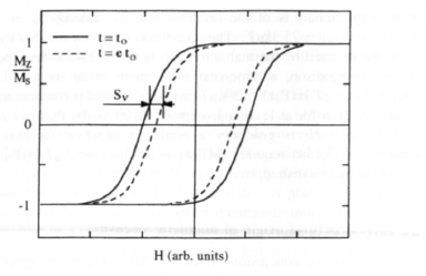
Figure 3.41. Magnetic viscosity and the fluctuation field. The time used to measure the loops is denoted by \(t\). In general, \(S_{\mathrm{v}}\) depends on \(H\).
Coherent Rotation
For aligned and interaction-free spherical Stoner–Wohlfarth particles (\(\Theta = 0\) in figure 3.19), one obtains by straightforward calculation the activation-energy expression
\(E = K_{1}V\left(1 + \frac{H}{H_{0}}\right)^{2}\). (3.140)
Here \(V\) is the physical volume of the particle and \(H_{0} = -H_{\mathrm{s}} = 2K_{1}/\mu_{0}M_{\mathrm{s}}\). This yields \(H_{\mathrm{f}}(E) = H_{0}(E/K_{1}V)^{1/2}\) and, with (3.134) and (3.138),
\(S_{\mathrm{v}} = \frac{1}{\mu_{0}M_{\mathrm{s}}}\sqrt{\frac{k_{\mathrm{B}}TK_{1}}{V\ln(\Gamma_{0}t_{0})}}\). (3.141)
Comparing this result with (3.139) we deduce \(V^{*} = V\sqrt{V_{\mathrm{th}}/V}\), where the 'thermal' volume \(V_{\mathrm{th}} = k_{\mathrm{B}}T\ln(\Gamma_{0}t_{0})/K_{1}\).
The behaviour of aligned Stoner–Wohlfarth particles shows (i) that the temperature dependence of the magnetic viscosity is generally nonlinear and (ii) that \(V^{*}\) is a temperature-dependent volume which has no real-space physical meaning.
Nonlinear Energy Landscapes
Equations (3.136) and (3.140) are easily generalized to the power law \(E = c_{0}(H - H_{\mathrm{s}})^{B}\), so that \(H_{\mathrm{f}}(E) = (E/c_{0})^{1/B}\). Besides the linear law (3.136) and the Stoner–Wohlfarth dependence (3.140), where \(B = 1\) and \(B = 2\), respectively, it describes for example strong domain-wall pinning and misaligned Stoner–Wohlfarth particles (both have \(B = 3/2\)). The temperature dependence of the viscosity scales as \(T^{1/B}\). For bulk ferromagnets, typical experimental exponents \(B\) vary from 1.0 to 1.4.
Explicit linearization of (3.134) yields
\(S_{\mathrm{v}} = k_{\mathrm{B}}T H_{\mathrm{f}}^{\prime}(k_{\mathrm{B}}T \ln(\Gamma_{0}t_{0}))\) (3.142)
where \(H_{\mathrm{f}}^{\prime}(E) = \mathrm{d}H_{\mathrm{f}}(E)/\mathrm{d}E\). The magnetic-viscosity coefficient is often written as \(S_{\mathrm{v}} = k_{\mathrm{B}}T/(\partial E / \partial H)\), but this expression obscures the fact that the temperature dependence of \(S_{\mathrm{v}}\) cannot be reduced to a linear \(k_{\mathrm{B}}T\) term. Equation (3.142) may also be used to discuss energy landscapes going beyond the simple power laws discussed here which are of potential interest, for example, in magnetic recording.
Magnetic Viscosity and Coercivity
In a few cases it is possible to ascribe magnetic viscosity to well defined mechanisms32. The coercivity of steels is largely determined by interstitial atoms such as carbon. The diffusive motion of the interstitial atoms gives rise to the diffusion after-effect. Physically, the domain-wall energies of carbon steels depend on the local carbon concentration, so that the application of an external magnetic field promotes a diffusive rearrangement of the carbon atoms and of the wall position until the total energy is minimized. This adaptation, also known as the Snoek effect, influences both magnetic and mechanical relaxations.
Magnetic viscosity increases with coercivity, and experiment shows that \(S_{\mathrm{v}}\) scales as \(H_{\mathrm{c}}^{x}\) for a wide range of metallic magnets, where \(x \approx 0.73\) (Wohlfarth 1984). A reversed nucleus of radius \(\delta_{\mathrm{B}}\) has an energy of order \(\gamma \delta_{\mathrm{B}}^{2} \approx K_{1} \delta_{\mathrm{B}}^{3}\) and an activation volume roughly proportional to \(\delta_{\mathrm{B}}^{3}\). This means that \(H_{\mathrm{c}} \propto K_{1}\), \(\delta_{\mathrm{B}} \propto 1/K_{1}^{1/2}\) and (3.139) yield the estimate \(S_{\mathrm{v}} \propto H_{\mathrm{c}}^{3/2}\). Magnetic-viscosity measurements on sintered Nd2Fe14B support this idea and provide a further proof that magnetic reversal in microsize grains proceeds by incoherent nucleation and not by coherent rotation.
Superparamagnetism
Random thermal fluctuations of the magnetization of small particles are significant when the anisotropy energy is within an order of magnitude of \(k_{\mathrm{B}}T\). As a result of these thermal fluctuations, the entire particle behaves like a huge paramagnetic spin (compare the ionic paramagnetism considered in section 2.2.4.1).
Consider aligned fine particles whose magnetization rotates coherently. There are two energy minima at \(M_{z} = \pm M_{\mathrm{s}}\) (figure 3.1) characterized by the
activation energies
\(E_{\pm}=K_{1}V\left(1 \pm \frac{H}{H_{0}}\right)^{2}\). (3.143)
To describe thermally activated transitions between the two minima we use the master equation
\(\frac{\mathrm{d}P_{+}}{\mathrm{d}t}=W_{-}P_{-}-W_{+}P_{+}\) (3.144a)
\(\frac{\mathrm{d}P_{-}}{\mathrm{d}t}=W_{+}P_{+}-W_{-}P_{-}\) (3.144b)
and assume that
\(W_{\pm}=\frac{1}{2\tau_{0}}\exp\left(-\frac{\Delta E_{\pm}}{k_{\mathrm{B}}T}\right)\). (3.145)
Taking into account the fact that \(p_{+}+p_{-}=1\) and \(M = M_{\mathrm{s}}(p_{+}-p_{-})\), we obtain the equation
\(\frac{\mathrm{d}M}{\mathrm{d}t}=-\Gamma(M - M_{\infty})\) (3.146)
having the solution \(M(t)=M_{0}+(M(0)-M_{\infty})\exp(-\Gamma t)\). Here
\(\Gamma=\frac{1}{\tau_{0}}\exp\left(-\frac{K_{1}V}{k_{\mathrm{B}}T}\left(1+\frac{H^{2}}{H_{0}^{2}}\right)\right)\cosh\left(\frac{\mu_{0}M_{\mathrm{s}}VH}{k_{\mathrm{B}}T}\right)\) (3.147)
and
\(M_{0}=M_{\mathrm{s}}\tanh\left(\frac{\mu_{0}M_{\mathrm{s}}VH}{k_{\mathrm{B}}T}\right)\) (3.148)
are the inverse relaxation time (relaxation rate) and the equilibrium magnetization, respectively. In the absence of magnetic fields, (3.147) reduces to the frequently used Arrhenius law
\(\Gamma=\frac{1}{\tau_{0}}\exp\left(-\frac{K_{1}V}{k_{\mathrm{B}}T}\right)\) (3.149)
which can also be written as \(\ln(\tau)\propto E_{0}/k_{\mathrm{B}}T\). Physically, it states that high-energy barriers yield exponentially increasing relaxation times.
In small particles, (3.144) gives rise to superparamagnetism. First, in very small particles the field \(H\) is unable to produce saturation. From (3.148) one obtains the \(K_{1}\)-independent equilibrium volume \(k_{\mathrm{B}}T/\mu_{0}M_{\mathrm{s}}H\) below which thermal activation dominates the Zeeman interaction. In fields of 1 T, the room-temperature equilibrium radius
\(R_{\mathrm{eq}}=\left(\frac{3k_{\mathrm{B}}T}{4\pi\mu_{0}M_{\mathrm{s}}H}\right)^{1/3}\) (3.150)
is about 1 nm for a wide range of ferromagnetic materials.
Second, (3.147) establishes a time \(t_{\mathrm{B}} \approx 1/\Gamma\) above which the zero-field magnetization is close to its equilibrium value zero and a superparamagnetic blocking radius \(R_{\mathrm{B}}(K_{1},T,t_{\mathrm{B}})\) below which the particles lose their remanent magnetization due to thermal excitations. From (3.149) it follows that
\(\frac{4\pi}{3}R_{\mathrm{B}}^{3}=\frac{k_{\mathrm{B}}T}{K_{1}}\ln\frac{t_{\mathrm{B}}}{\tau_{0}}\) (3.151)
where the time \(t_{\mathrm{B}}\) depends on the problem in question. This equation is usually written in terms of the blocking volume \(V_{\mathrm{B}}\) as
\(t_{\mathrm{B}}=\tau_{0}\exp\frac{k_{1}V_{\mathrm{B}}}{k_{\mathrm{B}}T}\). (3.152)
Thus, comparison of \(R_{\mathrm{B}}\) for 100 s and 10000000 years yields an increase of \(R_{\mathrm{B}}\) by less than 30%. Typical room-temperature blocking radii are 4 nm and 2 nm for cobalt and Nd2Fe14B, respectively.
Alternatively, one can use (3.149) to define a blocking or freezing temperature below which the magnetization ceases to change very much. This freezing is a universal phenomenon, common not only to fine-particle magnets but also to magnetic rocks, spin glasses and recording media. High recording densities are relentlessly reducing the volume of the medium in which each bit is recorded and recording technology has advanced towards the point where the superparamagnetic behaviour of individual grains will limit further progress.
Magnetic and Structural Length Scales
In this chapter we have encountered various length scales. Crystal-field interactions, spin–orbit coupling and exchange depend on the atomic structure and determine intrinsic materials parameters such as \(A\) and \(K_{1}\). By comparison, extrinsic properties are determined on a micromagnetic scale (table 3.9).
Table 3.9. A summary of the micromagnetic length scales (in nm). Note that there are no simple scaling laws for \(R_{\mathrm{eq}}\) and \(R_{\mathrm{B}}\).
| Length | Equation | Scaling | Fe | Nd2Fe14B |
|---|---|---|---|---|
| \(l_{\mathrm{ex}}\) | (3.71) | \(l_{\mathrm{ex}}\) | 1.5 | 1.9 |
| \(l_{\mathrm{coh}}\) | (3.91) | \(\sqrt{24}l_{\mathrm{ex}}\) | 7 | 9 |
| \(\delta_{\mathrm{B}}\) | (3.67) | \(\pi l_{\mathrm{ex}}/\kappa\) | 40 | 3.9 |
| \(R_{\mathrm{sd}}\) | (3.70) | \(36\pi l_{\mathrm{ex}}\) | 6 | 107 |
| \(R_{\mathrm{eq}}\) | (3.150) | — | 0.8 | 0.9 |
| \(R_{\mathrm{B}}\) | (3.151) | — | 8 | 2 |
True permanent magnetism means that \(K_{1}\) dominates on a micromagnetic scale. In particular, the critical single-domain radius \(R_{\mathrm{sd}}\), scaling as \(\kappa\), is much
larger than the Bloch-wall thickness \(\delta_{\mathrm{B}}\), the exchange length \(l_{\mathrm{ex}}\), the coherence length \(l_{\mathrm{coh}}\), the equilibrium radius \(R_{\mathrm{eq}}\) and the blocking radius \(R_{\mathrm{B}}\). In practice, coercivity and remanence are determined by structural inhomogeneities whose size is comparable to the domain-wall width and even in perfect ellipsoids of revolution the relevant structural length scale, namely \(R_{\mathrm{coh}}\), is much smaller than \(R_{\mathrm{sd}}\). As a consequence, the critical single-domain size is largely irrelevant in the context of major hysteresis loops33.


