2.3 Magnetic Order: A Comprehensive Overview
The first part of this section is devoted to the atomic origin of the zero-temperature ferromagnetic order, whereas the second part shows how thermal excitations destroy the magnetization at the Curie temperature. Here we focus on the Heisenberg-type interactions, whereas the itinerant ferromagnetism of metallic 3d magnets will be dealt with in section 2.4.
Understanding Zero-Temperature Magnetic Order
Figure 1.6 showed the three basic types of zero-temperature magnetic order: ferromagnetism, ferrimagnetism and antiferromagnetism. There exist more complicated varieties such as canted antiferromagnetism in α-Fe2O3, helimagnetism in many rare earths and spin-density wave antiferromagnetism in Cr. In ferromagnets, such as Fe, Nd2Fe14B and CrO2, the net atomic magnetization points in the same direction everywhere in a domain in the crystal and the net magnetization is obtained by adding all atomic moments. Ferrimagnetic order, which implies the existence of at least two antiparallel magnetic sublattices, is observed in transition-metal oxides such as Fe3O4, Y3Fe5O12 and BaFe12O19, and in rare-earth intermetallics such as Dy2Fe17. Antiferromagnets have equal sublattices and vanishing net magnetisation at all temperatures. In fact, many transition-metal oxides and halides such
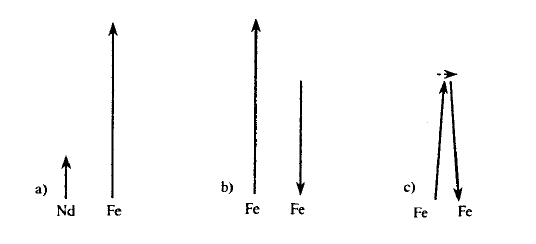
Figure 2.23. Magnetic order in Nd2Fe14B, BaFe12O19 and αFe2O3. The structures are ferromagnetic, ferrimagnetic and canted antiferromagnetic respectively.
as MnO, CoO, NiO, FeF2 and MnCl2 are antiferromagnets and cannot be used as permanent magnets, although those with a high Néel temperature are sometimes used in multilayers to fix the magnetization direction of an adjacent ferromagnetic layer by exchange coupling (exchange bias). Examples of magnetic order are shown in figure 2.23.
In terms of ionic magnetism, magnetic order is the inter-atomic alignment of localized magnetic moments due to a Heisenberg-like exchange interaction. The sign of the exchange parameter decides whether the coupling is ferromagnetic (J > 0) or antiferromagnetic (J < 0), whereas the magnitudes of the exchange constants determine the critical temperature below which magnetic ordering occurs. This picture applies to rare-earth atoms in metals and non-metals but is also realized in 3d oxides. Magnetic order in 3d metals is closely linked to itinerant moment formation (section 2.4), but we will see that some features of localized magnetism survive in late 3d magnets. The magnetization of transition-metal-rich rare-earth intermetallics, such as Nd2Fe14B, is dominated by the transition-metal sublattice, so that the rare-earth contribution is of secondary importance.
Superexchange
Magnetic oxides of the late 3d elements, such as Fe3O4, consist of large O2− ions and comparatively small transition-metal anions such as ferric iron (Fe3+) and ferrous iron (Fe2+) (table 5.1). Charge neutrality leads to units such as FeO and Fe2O3 containing Fe2+ and Fe3+, respectively. The exchange between well localized 3d moments is often—but not always—negative, which explains the widespread occurrence of antiferromagnetism or ferrimagnetism in transition-metal oxides.
Since the magnetic ions are well separated by the large oxygen anions, the direct exchange between the transition-metal ions is negligible in most oxides. However, oxygen ions are able to mediate some hopping between the
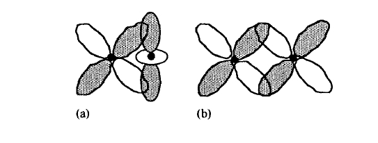
Figure 2.24. Overlapping non-s orbitals characterized by (a) zero and (b) non-zero overlap (hopping). White and grey areas denote positive and negative wavefunctions, respectively.
magnetic ions and give rise to superexchange. The sign of the effective exchange interaction is given by the semiphenomenological Goodenough–Kanamori rules (Anderson 1963, Goodenough 1963).
(i) When two cations have lobes of occupied 3d orbitals which point towards each other, giving large overlap and hopping integrals, the exchange is antiferromagnetic.
(ii) When two cations have an overlap integral which is zero by symmetry, the exchange is ferromagnetic.
A theoretical justification of the Goodenough–Kanamori rules is provided by treating inter-atomic hopping as a small perturbation of the leading intra-atomic energies. The presence of intermediary ions makes the calculation complicated, but essentially one obtains an effective exchange constant of the type (2.60). The main difference is a modification of the hopping integral (2.45), which now depends on the symmetry and coordination of the non-s orbitals involved (figure 2.24). The direct exchange \(J_{D}\) is always positive, but it is comparatively small and the kinetic exchange \(-2\Delta T^{2}/U \approx -2T_{0}^{2}/U\) dominates (first rule) unless \(T_{0}\) is zero by symmetry (second rule). The first rule applies, for example, when d orbitals (\(e_{g}\) in octahedral coordination) point towards each other with a near \(180^{\circ}\) T–O–T bond angle.
If the sublattice structure of an oxide is known, then the magnetic moment is easily obtained from the quenched spin-only moments. For example, magnetite (Fe3O4) crystallizes in a cubic spinel structure (figure 5.3) and has two antiparallel sublattices A and B which are coupled via a \(125^{\circ}\) A–O–B superexchange bond (figure 5.3). Fe3+ ion per formula unit belongs to the sublattice A, while the second Fe3+ ion and the Fe2+ ion form the sublattice B. With the ionic moments \(m(Fe^{2+}) = 4\ \mu_{B}\) and \(m(Fe^{3+}) = 5\ \mu_{B}\) we obtain the net magnetic moment \(4\ \mu_{B}\), which is close to the experimental value \(4.1\ \mu_{B}\). Magnetic moments for a few oxides are quoted in table 2.8. A detailed discussion is given in section 5.1.
Table 2.8. Magnetic structures and moments (per formula unit at \(T = 0\)) of some oxides.
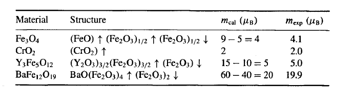
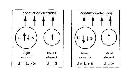
Figure 2.25. Intersublattice exchange in rare-earth transition-metal intermetallics.
4f Magnetism
The magnetization of transition-metal-rich rare-earth intermetallics, such as SmCo5, Sm2Fe17N3 and Nd2Fe14B, is largely determined by the transition-metal sublattice. The interaction between the rare-earth atoms is practically negligible, but the rare-earth transition-metal interaction, mediated by the rare-earth 5d and 6s conduction electrons, determines the inter-sublattice coupling and enhances the Curie temperature. It turns out that the inter-sublattice coupling of the spins is antiferromagnetic if the rare earth's partner is a late 3d element. Since Hund's rules predict the rare-earth spin and total moments to be antiparallel for the light lanthanides but parallel for the heavy lanthanides, the coupling between the rare-earth and transition-metal sublattice moments is ferromagnetic for the light rare earths but antiferromagnetic for the heavy rare earths (Figure 2.25). For this reason, permanent magnets contain light rare earths such as Nd and Sm, whereas magneto-optical storage media, which have to exhibit a small net magnetization to reduce magnetostatic demagnetizing effects, contain heavy rare earths such as Dy.
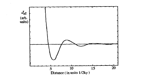
Figure 2.26. Oscillatory RKKY exchange.
Indirect Exchange
Exchange interactions between localized moments in metals are mediated by conduction electrons. The simplest coupling mechanism is the Ruderman–Kittel–Kasuya–Yosida (RKKY) interaction. Consider two spins \(S_{1}\) and \(S_{2}\) localized at \(R_{1} = 0\) and \(R_{2} = R\), respectively, in a free-electron gas. A given conduction electron labelled \(k_{\sigma}\) feels a spin-dependent potential \(V_{\sigma, i}(\boldsymbol{r}) = \pm V_{0}\delta(\boldsymbol{r} - R_{i})\) where the sign refers to the relative spin orientation between the localized and delocalized electrons. The energy of the free-electron gas is obtained by standard perturbation theory and depends on whether the localized spins \(S_{1}\) and \(S_{2}\) are parallel or antiparallel. In other words, the distance dependence of the RKKY interaction is given by the \(R\)-dependent energy difference between the parallel and antiparallel configurations.
The starting point is the Schrödinger equation
\(-\frac{\hbar^{2}}{2m_{e}} \nabla^{2}\psi + E_{0}\psi + V_{\sigma}(\boldsymbol{r})\psi = E\psi\) (2.102)
which yields the perturbed one-electron energies \(E_{k\sigma}\). The first-order correction \((1/V) \int V_{\sigma}(\boldsymbol{r}) d\boldsymbol{r}\) may be neglected, since the contributions of the \(\uparrow\) and \(\downarrow\) free electrons cancel each other. The second-order correction is given by
\(\Delta E_{k\sigma} = -\sum_{\boldsymbol{k}'} \frac{\langle\psi_{k\sigma}|V_{\sigma}|\psi_{k'0}\rangle\langle\psi_{k'0}|V_{\sigma}|\psi_{k\sigma}\rangle}{E_{k'0} - E_{k0}}\) (2.103)
where \(\psi_{k\sigma}(\boldsymbol{r}) = V^{-1/2} \exp(i\boldsymbol{k} \cdot \boldsymbol{r})\). Replacing the quasi-continuous sum (2.103) by an integral, \(\sum_{\boldsymbol{k}'} = V/8\pi^{3} \int d\boldsymbol{k}'\), and consulting appendix A5.3 we find
\(\Delta E_{k\sigma} = -\frac{m_{e}}{2\pi V\hbar^{2}} \int \frac{\cos(k|\boldsymbol{r} - \boldsymbol{r}'|)}{|\boldsymbol{r} - \boldsymbol{r}'|} \text{e}^{i\boldsymbol{k} \cdot (\boldsymbol{r} - \boldsymbol{r}')}V_{\sigma}(\boldsymbol{r})V_{\sigma}(\boldsymbol{r}') d\boldsymbol{r} d\boldsymbol{r}'\). (2.104)
The integrations in this equation are trivial, since \(V_{\sigma}(r)\) consists of two \(\delta\) functions. Depending on \(k\) and \(r - r'\) the one-electron corrections exhibit an oscillatory behaviour.
The total energy of the perturbed free-electron gas is obtained from (2.104) by integrating over all occupied \(k_{\sigma}\) states (\(k \leq k_{\text{F}}\)). After a short calculation we obtain
\(\Delta E = -\frac{m_{e}k_{\text{F}}^{4}}{\pi^{3}\hbar^{2}} \int F(2k_{\text{F}}|r - r'|)V_{\sigma}(r)V_{\sigma}(r') dr dr'\) (2.105)
where
\(F(x) = \frac{\sin x - x \cos x}{x^{4}}\). (2.106)
Evaluating \(\Delta E\) for \(V_{\sigma}(r) = V_{0}\delta(r) \pm V_{0}\delta(r - R)\), that is for \(S_{1} = \pm S_{2}\), yields the oscillatory RKKY exchange
\(\mathcal{J}_{\text{eff}} = \frac{m_{e}k_{\text{F}}^{4}V_{0}^{2}}{\pi^{3}\hbar^{2}} \frac{\sin(2k_{\text{F}}R) - 2k_{\text{F}}R \cos(2k_{\text{F}}R)}{(2k_{\text{F}}R)^{4}}\) (2.107)
shown in figure 2.26. RKKY oscillations are akin to the Friedel electron-density oscillations caused by impurities in metals and indicate that the spatial resolution of free-electron waves is of the order of \(1/k_{\text{F}}\). Alternatively, they may be interpreted as rudimentary electron shells formed around impurities.
The RKKY mechanism gives a qualitative account of the inter-atomic exchange coupling between localized moments such as rare-earth ions in metals and, more approximately, between 3d atoms in metals14. The qualitative character of (2.107) reflects the perturbative character of the approach and the approximation of hybridizing s, p and d wavefunctions by a free-electron gas.
Magnetic Interactions and The Number of d Electrons
There is a general trend towards antiferromagnetic interactions between half-filled shells, whereas the magnetic coupling near the beginning of the 3d series and near the end may be ferromagnetic. A simple local-moment explanation of the antiferromagnetism associated with half-filled shells is based on the energy gain due to inter-atomic hopping. Hopping is greatly enhanced when the spins are antiparallel, whereas parallel spins must obey the Pauli principle.
An alternative explanation is provided by the diatomic model Hamiltonian of section 2.1.5
\(\mathcal{H}_{\text{FM}} = \begin{pmatrix} \pm V & T \\ T & \pm V \end{pmatrix}\) (2.108a)
and
\(\mathcal{H}_{\text{AFM}} = \begin{pmatrix} \pm V & T \\ T & \mp V \end{pmatrix}\). (2.108b)
14 Delocalized ground-state wavefunctions (section 2.4.2) do not exclude localized excitations in itinerant magnets and for large distances these excitations may be considered as point-like.
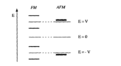
Figure 2.27. Ferromagnetic and antiferromagnetic level splittings for the diatomic model (2.108).
These equations, where the diagonal matrix elements give the spin-dependent local exchange potential and the parameter \(T\) is the inter-atomic hopping, may be interpreted as rudimentary band-structure Hamiltonians. Note that the ferromagnetic (FM) potential \(\pm V\) is spin-polarized but site-independent, whereas in the antiferromagnetic case (AFM) a given spin feels opposite exchange potentials on neighbouring sites. Equation (2.108) amounts to a Stoner-type one-electron exchange splitting (section 2.1.6.1), where the energy levels are occupied by independent electrons.
Diagonalizing (2.108) we find the energy levels shown in figure 2.27. The ferromagnetic eigenstates are \(-V \pm T\) and \(+V \pm T\), whereas the antiferromagnetic energy levels are double degenerate:
\(E_{\text{AFM}} = \pm\sqrt{V^{2} + T^{2}}\). (2.109)
We see that for nearly empty shells (one electron in this simple model) the ferromagnetic potential yields the lower energy, whereas half-occupied orbitals (two electrons) yield antiferromagnetism. This band-filling dependence of the effective exchange is related to the Bethe–Slater–Néel curve (figure 2.8) and explains why Cr and Mn are not ferromagnets.
Exploring Finite-Temperature Magnetic Models and Approximations
An important problem in solid-state magnetism is the temperature dependence of the spontaneous magnetization. In particular, it is important to know the Curie temperature above which the spontaneous magnetization vanishes. To derive temperature-dependent quantities such as magnetization and susceptibility it is sufficient to calculate the partition function \(Z = \text{Tr}(\exp(-\mathcal{H}/k_{\text{B}}T))\) or, in classical statistics, \(\sum \exp(-\mathcal{H}/k_{\text{B}}T)\)15. However, the calculation of \(Z\) is
15 See appendix A4.
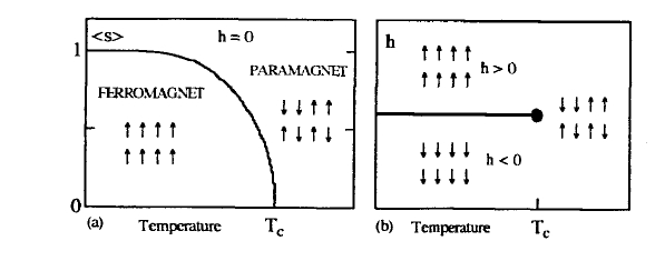
Figure 2.28. Ising ferromagnet: (a) the zero-field or spontaneous magnetization as a function of temperature calculated in the mean-field approximation (section 23.2.3) and (b) the field-versus-temperature phase diagram.
generally very difficult, because the number of spin configurations over which the trace or sum extends increases exponentially with the number \(N\) of atomic spins. For this reason it is necessary to use simplifying models and approximations.
In this subsection we investigate the temperature dependence of the spontaneous magnetization of local-moment magnets. Some discussion of phase transitions is given in appendix A4.4. The temperature dependence of the magnetization of itinerant magnets and the finite-temperature behaviour of the magnetic anisotropy will be dealt with in sections 2.4.3 and 3.1.5, respectively. A particularly useful approach set out by Weiss (1907) is the thermodynamical molecular-field or mean-field approximation, where the inter-atomic interaction is replaced by an effective field acting on the individual spins. Originally, the mean field was believed to originate from a magnetostatic interaction, the Weber–Ewing theory of ferromagnetism, but later it became clear that the ferromagnetic coupling must arise from the much stronger quantum-mechanical exchange.
Ising and Heisenberg Models
The simplest model describing phase transitions is the spin-\(\frac{1}{2}\) Ising model. It is defined by the Hamiltonian
\(\mathcal{H} = -\frac{1}{2} \sum_{i,k=1}^{N} \mathcal{J}_{ik}s_{i}s_{k} - \sum_{i=1}^{N} h_{i}s_{i}\) (2.110)
where a given microscopic configuration is characterized by a set of phase-space variables \((s_{1}, s_{2}, \ldots, s_{N})\) with two states \(s_{i} = \pm 1\) per site (Ising 1925). In a magnet, the local configurations \(s_{i} = \pm 1\) describe spin-up (\(\uparrow\)) and spin-down (\(\downarrow\)) states, respectively. Up to a constant prefactor, \(h_{i}\) is the magnetic field acting on the \(i\)th spin and the exchange constants \(\mathcal{J}_{ik} = \mathcal{J}(r_{i} - r_{k})\) parametrize the inter-atomic exchange responsible for the phase transition16. Positive and negative values of \(J_{ik}\) indicate ferromagnetic and antiferromagnetic exchange, respectively. Note, furthermore, that there is no difference between the classical and quantum-mechanical Ising models, since the \(z\)-components of spin operators commute. As discussed in appendix A4, the Ising model is not restricted to magnetism; it can also be applied to alloys and gases in metals.
Figure 2.28 illustrates the finite-temperature magnetism of the ferromagnetic Ising model. At zero temperature, all spins are parallel, whereas above \(T_{\text{C}}\) the spins are paramagnetic. Although the Ising model is conceptually very simple, its solution, that is the calculation of the partition function, is complicated in most cases. For nearest-neighbour interactions, the ferromagnetic Ising model has been solved in one and two dimensions, by Ising (1925) and Onsager (1944), respectively.
A disadvantage of the Ising model is that it contains only two states per site. For real materials it is often better to use the Heisenberg model
\(\mathcal{H} = -\frac{2}{\hbar^{2}} \sum_{i<k} J_{ik} \hat{S}_{i} \cdot \hat{S}_{k} – \frac{g\mu_{\text{B}}\mu_{0}}{(g – 1)\hbar} \sum_{i} H_{i} \cdot \hat{S}_{i}\) (2.111)
This Hamiltonian differs from (2.62) by the inclusion of the ionic Landé factor \(g\). Note that \(\hbar\) is often omitted in equations such as (2.111)—the angular momentum is then taken in units of \(\hbar\) rather than \(J\ s\).
As in the Ising model, the sign of \(J_{ik}\) in (2.111) decides whether the interaction is ferromagnetic (\(J_{ik} > 0\)) or antiferromagnetic (\(J_{ik} < 0\)). A further complication is the quantum-mechanical character of the Heisenberg model, which arises from the fact that the spin operators \(\hat{S}_{x}\), \(\hat{S}_{y}\) and \(\hat{S}_{z}\) do not commute.
The n-vector Model
A classical generalization of the Heisenberg and Ising models is the \(n\)-component vector spin model or \(n\)-vector model. The model Hamiltonian is
\(\mathcal{H} = -\frac{1}{2} \sum_{ik} J_{ik} s_{i} \cdot s_{k} - \sum_{i} h_{i} \cdot s_{i}\) (2.112)
where the spin variables \(s_{i} = s_{ix}e_{x} + s_{iy}e_{y} + \cdots + s_{in}e_{n}\) obey \(s_{i}^{2} = 1\). It is worth emphasizing that the number \(n\) of spin components is independent of the dimensionality \(d\) of the lattice on which the atomic spins are arranged. In (2.112), the lattice dimensionality is contained in the exchange parameters \(J_{ik}\).
Putting \(n = 1\) reproduces the Ising model, whereas \(n = 2\) and \(n = 3\) define the classical planar or \(XY\) and Heisenberg models, respectively. In familiar notation the spin variables are \(s_{i} = \sin\theta_{i}e_{x} + \cos\theta_{i}e_{z}\) and
16 There are different ways of defining the \(J_{ik}\). In (2.110) the prefactor \(1/2\) has been chosen to assure that the exchange energy per bond equals \(\pm J_{ik}\).
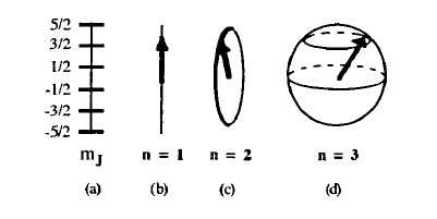
Figure 2.29. Spin configurations (a) the \(J = 5/2\) Heisenberg model, (b) the Ising model, (c) the planar model and (d) the classical Heisenberg model. Classical Heisenberg spins (d) differ from quantum-mechanical Heisenberg spins (a) by having a continuous number of spin or moment projections onto the \(z\)-axis.
\(s_{i} = \sin\theta_{i} \cos\phi_{i} e_{x} + \sin\theta_{i} \sin\phi_{i} e_{y} + \cos\theta_{i} e_{z}\) in the respective models. The limit \(n = \infty\) is called the spherical model and it can be shown that the \(n = 0\) vector spin model describes a self-avoiding polymer chain (de Gennes 1979). Figure 2.29 shows local spin configurations of some spin models. Note that the spherical model can be solved exactly in more than two dimensions (see appendix A4.5).
The Mean-field Solution of The Ising Model
To study the ferromagnetic phase transition we replace (2.110) by
\(\mathcal{H}_{\text{MF}} = -\sum_{i} h_{i,\text{eff}}s_{i}\) (2.113)
where \(h_{i,\text{eff}}\) is the mean field acting on the \(i\)th spin. The advantage of this approximate Hamiltonian is that it reduces the original problem to the treatment of an ensemble of independent spins. As a consequence, the partition function factorizes as \(\mathcal{Z} = \mathcal{Z}_{1}\mathcal{Z}_{2}\cdots\mathcal{Z}_{N}\), where \(\mathcal{Z}_{i} = 2\cosh(h_{i,\text{eff}}/k_{\text{B}}T)\).
The starting point of the calculation of \(h_{i,\text{eff}}\) is the identity
\(s_{i}s_{k} = s_{i}\langle s_{k}\rangle + \langle s_{i}\rangle s_{k} - \langle s_{i}\rangle\langle s_{k}\rangle + K_{ik}\) (2.114)
where the term \(K_{ik} = (s_{i} - \langle s_{i}\rangle)(s_{k} - \langle s_{k}\rangle)\) describes spin correlations. The average \(\langle s_{i}\rangle\langle s_{k}\rangle\) can be omitted, because it does not contribute to the microstate summation over all spin variables \(s_{i} = \pm 1\) but merely yields a physically irrelevant prefactor in the partition function. By contrast, the matrix \(K_{ik}\) contains unaveraged spin contributions and needs further consideration. The main assumption of the mean-field theory is to replace \(K_{ik}\) by its average \(\langle K_{ik}\rangle = \Gamma_{ik}\), so that the \(K_{ik}\) term in (2.114) becomes negligible17. Putting
17 Note that the widely used replacement of \(J_{ik}s_{i}s_{k}\) by \(J_{ik}s_{i}\langle s_{k}\rangle\) fails to reproduce the mean-field approximation by a factor of two. An alternative derivation of the correct factor is based on the variational free energy approach outlined in appendix A4.3.
Reduced field \(h/k_{\text{B}}T\)
Figure 2.30. A graphical solution of the mean-field equation (2.116).
the remainder of (2.114) into (2.110) yields
\(h_{i,\text{eff}} = h_{i} + \sum_{k} J_{ik}\langle s_{k}\rangle\) (2.115a)
or
\(h_{i,\text{eff}} = h_{i} + h_{i,\text{MF}}\). (2.115b)
The mean-field equation of state, that is the magnetization as a function of temperature and magnetic field, is obtained from the partition function: \(\langle s_{i}\rangle = k_{\text{B}}T \ln \mathcal{Z}/\partial h_{i} = \tanh(h_{i,\text{eff}}/k_{\text{B}}T)\). Since the effective field \(h_{i,\text{eff}}\) depends on \(\langle s_{i}\rangle\), this equation has to be solved self-consistently.
In homogeneous magnets, the \(J_{ik}\) and consistently exhibit translational symmetry, so that \(\sum_{k} J_{ik}\langle s_{k}\rangle = z\mathcal{J}_{0}\). Here \(z\) is the number of neighbours coupled to \(s_{i}\) by the exchange interaction and \(\mathcal{J}_{0}\) denotes the average exchange between the interacting neighbours. Thus
\(\langle s\rangle = \tanh\frac{h + z\mathcal{J}_{0}\langle s\rangle}{k_{\text{B}}T}\). (2.116)
Putting \(h = 0\) in this equation yields the spontaneous magnetization. Graphically, the solution of (2.116) is obtained by plotting \(\langle s\rangle\) and \(\tanh(z\mathcal{J}_{0}\langle s\rangle/k_{\text{B}}T)\) versus \(h/k_{\text{B}}T\). In figure 2.30, the two functions are shown as full and dashed curves, respectively. Note that the slope of the dashed lines equals the ratio of thermal energy, \(k_{\text{B}}T\), to inter-atomic exchange, \(z\mathcal{J}_{0}\).
From figure 2.30 we see that there is a temperature, namely the Curie temperature \(T_{\text{C}} = z\mathcal{J}_{0}/k_{\text{B}}\), above which there is only one paramagnetic solution of (2.116), \(\langle s\rangle = 0\) (compare figure 2.28). Below \(T_{\text{C}}\) there are three solutions: an unstable paramagnetic solution \(\langle s\rangle = 0\) and two stable ferromagnetic solutions characterized by non-zero spontaneous magnetisation \(M_{s}\): \(\langle s\rangle = \pm M_{s}/M_{0}\). Just below \(T_{\text{C}}\) the spontaneous magnetization is very small, so that the Curie< temperature is obtained by putting \(h = 0\) in (2.116) and expanding the remainder into powers of \(\langle s\rangle\). The result is \(\langle s\rangle = z\mathcal{J}_{0}\langle s\rangle/k_{\text{B}}T_{\text{C}}\) or
\(T_{\text{C}} = \frac{z\mathcal{J}_{0}}{k_{\text{B}}}\). (2.117)
It is normal to restrict consideration to the positive branch of the spontaneous magnetization, which yields the phase diagram of figure 2.28(a). Below \(T_{\text{C}}\), there is a line of first-order phase transitions separating the \(\uparrow\) and \(\downarrow\) phases (figure 2.28(b)), and at \(T_{\text{C}}\) the order-parameter difference \(2M_{\text{s}}\) vanishes. This behaviour at the critical point \(T = T_{\text{C}}\) and \(h = 0\) is known as a second-order phase transition.
Two-sublattice Ising Magnets
Negative exchange parameters \(J_{ik}\) favour an antiparallel spin alignment between the interacting neighbours (Néel 1932, 1948) and describe antiferromagnetism. It is not always possible to find a spin configuration which minimizes the energy of all spin pairs simultaneously, but often the consideration of two sublattices \(r_{i}\) and \(r_{i}^{\prime}\) having the respective sublattice magnetizations \(\langle s\rangle\) and \(\langle s^{\prime}\rangle\) is a good starting point. In the absence of intra-sublattice interactions one obtains the mean-field equations
\(\langle s\rangle = \tanh((h - z\mathcal{J}_{0}\langle s^{\prime}\rangle)/k_{\text{B}}T)\) (2.118a)
\(\langle s^{\prime}\rangle = \tanh((h - z\mathcal{J}_{0}\langle s\rangle)/k_{\text{B}}T)\). (2.118b)
Putting \(h = 0\) and using the ansatz \(\langle s^{\prime}\rangle = -\langle s\rangle\) yields a second-order phase transition at the Néel temperature \(T_{\text{N}} = z|\mathcal{J}_{0}|/k_{\text{B}}\), below which spins on nearest-neighbour sites belong to different sublattices with opposite spin directions. A more complicated situation is encountered if the inter-sublattice exchange \(\mathcal{J}_{0}^{\prime}\) is accompanied by some intra-sublattice exchange \(\mathcal{J}_{0}^{\prime\prime}\). Then the (antiferromagnetic) Néel temperature \(k_{\text{B}}T_{\text{N}} = \mathcal{J}_{0}^{\prime} - \mathcal{J}_{0}^{\prime\prime}\) is different from the paramagnetic Néel temperature \(\theta_{\text{N}} = \mathcal{J}_{0}^{\prime} + \mathcal{J}_{0}^{\prime\prime}\) deduced from the temperature dependence of the susceptibility. Only in the simplest antiferromagnets does \(\theta_{\text{N}} = -T_{\text{N}}\).
The mean-field Solution of The \(n\)-vector Model
The mean-field treatment of the \(n\)-vector model reduces to the consideration of isolated spins in the effective field \(h_{\text{eff}} = z\mathcal{J}_{0}\langle s\rangle\). The starting point is the one-spin partition function \(Z = \int \exp(h_{\text{eff}} \cdot s/k_{\text{B}}T) \text{d}S\), where the integration is performed over the surface of an \(n\)-dimensional sphere (figure 2.29). Since the mean field vanishes at \(T_{\text{C}}\), the partition function can be expanded in powers of \(h_{\text{eff}}\). This procedure yields
\(T_{\text{C}} = \frac{z\mathcal{J}_{0}}{nk_{\text{B}}}\). (2.119)
Putting \(n = 1\) reproduces the Curie temperature (2.117) of the Ising model, whereas the classical Heisenberg model is described by \(n = 3\).
An interesting point is the influence of magnetic anisotropy on the Curie temperature. The starting point is the mean-field Hamiltonian
\(\mathcal{H}_{\text{MF}} = -z\mathcal{J}_{0}s_{z}(s_{z}) + Ks_{z}^{2}\) (2.120)
where \(K = K_{1}\Omega_{\text{at}}\) is the anisotropy energy per magnetic atom. Since permanent magnets are characterized by \(K \ll z\mathcal{J}_{0}\), we can treat the anisotropy as a small perturbation and obtain
\(T_{\text{C}} = \frac{z\mathcal{J}_{0}}{nk_{\text{B}}} + \frac{2(n - 1)}{n(n + 2)k_{\text{B}}}K\). (2.121)
This equation leads to the estimate that an anisotropy of order \(1\ \text{MJ}\ \text{m}^{-3}\) yields a Curie-temperature shift of about \(1\ \text{K}\) in Heisenberg magnets. By comparison, (2.119) shows that the Curie temperature of the ideally anisotropic Ising model is as much as three times higher than that of the classical Heisenberg model. This explains why the (isotropic) Heisenberg model rather than the (anisotropic) Ising model is used to understand the Curie temperature of permanent magnets which are intrinsically anisotropic.
The Quantum-mechanical Heisenberg Model
The derivation of the mean-field Curie temperature is similar to the treatment of the Ising model. The main difference is that the hyperbolic tangent appearing in (2.116) has to be replaced by the appropriate Brillouin functions (2.94). The calculation yields the molecular field
\(\mathcal{H}_{\text{MF}} = \frac{2z\mathcal{J}_{0}(g - 1)^{2}(\vec{J})}{h g\mu_{\text{B}}\mu_{0}}\) (2.122)
and the mean-field Curie temperature
\(T_{\text{C}} = z\mathcal{J}_{0}\frac{2(g - 1)^{2}J(J + 1)}{3k_{\text{B}}}\). (2.123)
The de Gennes factor \(G = (g - 1)^{2}J(J + 1)\) arises from the relation \(\vec{S} = (g - 1)\vec{J}\) derived in section 2.2.2.3 and indicates that the exchange field acts on the spin only. If the orbital moment is quenched, then (2.111) reduces to (1.17)
\(T_{\text{C}} = z\mathcal{J}_{0}\frac{2S(S + 1)}{3k_{\text{B}}}\). (2.124)
It is worth noting that the parameter \(\mathcal{J}_{0}\) appearing in this equation is different to the one in (2.119)—the former refers to classical spins.
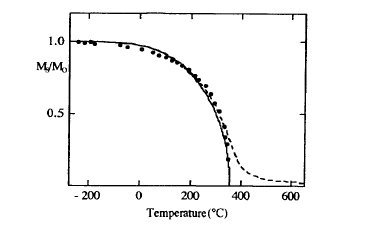
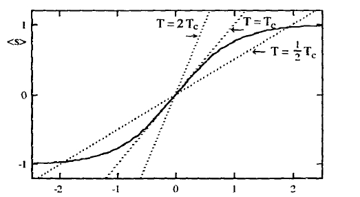
Figure 2.31. Mean-field magnetization of nickel: \(H = 0\) (full curve) and \(\mu_{0}H = 10\ \text{T}\) (dashed curve). The spin is taken as \(S = 1/2\).
The full curve in figure 2.31 shows the spontaneous magnetization of the Heisenberg model \(S = 1/2\) and \(g = 2\), whereas the dashed curve shows the mean-field magnetization in a field \(\mu_{0}H = 10\ \text{T}\). The parameter \(\mathcal{J}_{0}\) has been chosen to reproduce the experimental Curie temperature of nickel. Note that the spin quantum number \(S = 1/2\) yields a quenched moment of \(1\ \mu_{\text{B}}\), whereas the observed nickel moment is only \(0.6\ \mu_{\text{B}}\). The reason for the existence of non-integer moments in metals is the itinerant character of the 3d electrons (section 2.4), which is incompatible with the local-moment character of the atomic spins considered in this section. Furthermore, there are deviations from the mean-field behaviour, both at very low temperatures and near \(T_{\text{C}}\) (section 2.3.3).
It is important to understand that the temperature dependence of the spontaneous magnetization shown in figure 2.31 is unrelated to the macroscopic alignment of magnetic domains. Domains are characterized by a local magnetization \(M(\mathbf{r}) = M_{\text{s}}\mathbf{e}_{r}\), where the spontaneous magnetization \(M_{\text{s}}\) is an average over a few atomic distances. Comparing the full and dashed curves in figure 2.31 we see that the magnitude of the magnetization, \(M_{\text{s}}\), is only weakly field dependent unless one is close to the Curie temperature.
Two-sublattice Heisenberg Magnets
Many magnetic materials are characterized by two magnetic sublattices, which affect the material's intrinsic properties (see e.g. figure 5.19). In particular, the paramagnetic Curie temperature \(\theta_{\text{p}}\), deduced from the high-temperature Curie-Weiss limit \(\chi \approx C/(T - \theta_{\text{p}})\), differs from the magnetic ordering temperature (critical temperature) \(T_{\text{C}}\). As mentioned in section 2.3.2.4, these two temperatures are obtained by linearizing the multi-sublattice mean-field
Table 2.9. Moments and Curie temperatures of some transition-metal-rich rare-earth intermetallics.
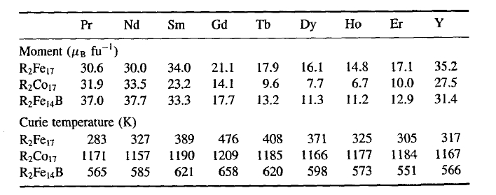
equations. Intra- and inter-sublattice interactions then appear as diagonal and non-diagonal coefficients in the linear equations, respectively, which form a square matrix. Basically, the respective temperatures \(T_{\text{C}}\) and \(\theta_{\text{p}}\) are obtained by diagonalizing and inverting the matrix, respectively. The paramagnetic Curie temperature can be written as \(\theta_{\text{p}} = \sum_{ik} c_{ik}J_{ik}\), where the coefficients \(c_{ik}\) are positive and depend on the structural and magnetic properties of the \(i\)th and \(k\)th sublattices. There is no general formula for \(T_{\text{C}}\), although there exist explicit Curie-temperature expressions for some simple many-sublattice magnets, such as the two-sublattice magnets discussed below and in section 5.1.1.
To a fair approximation, rare-earth permanent magnets such as \(Nd_{2}Fe_{14}B\) and hexagonal ferrites such as \(BaFe_{12}O_{19}\) consist of two sublattices coupled by ferromagnetic and antiferromagnetic interactions, respectively18. Table 2.9 shows the moments and Curie temperatures of some rare-earth transition-metal intermetallics. Although the leading contributions to both quantities are provided by the transition-metal sublattices, there is a systematic dependence on the rare-earth constituent. First, we note that the net moments of the compounds containing heavy rare earths are smaller than those of the isostructural compounds containing light rare earths. This is due to the fact that the intersublattice coupling is ferromagnetic and antiferromagnetic for the light and heavy rare earths, respectively (section 2.3.1.2). Second, it is striking that the Curie temperature is largest for the rare earths around gadolinium in the middle of the series. This is a finite-temperature two-sublattice effect.
The starting point is the two-sublattice Hamiltonian
\(\mathcal{H}^{\prime} = -\sum_{ij} J_{\text{TT}}\hat{S}_{i} \cdot \hat{S}_{j} - \sum_{ab} J_{\text{RR}}(g - 1)^{2}\hat{J}_{a} \cdot \hat{J}_{b} - \sum_{ia} J_{\text{RT}}(g - 1)\hat{S}_{i} \cdot \hat{J}_{a} - 2h\mu_{\text{B}}\mu_{0}H \cdot \sum_{i} \hat{S}_{i} - gh\mu_{\text{B}}\mu_{0}H \sum_{a} \hat{J}_{a}\) (2.125)
18 The approximate character of the two-sublattice approach is due to the presence of more than two non-equivalent sites in many materials.
where \(\mathcal{H}^{\prime} = \mathcal{H}\hbar^{2}\) and the subscripts T and R refer to the transition-metal and rare-earth sublattices, respectively19. The interacting rare-earth and transition-metal neighbours are characterized by the operators \(\hat{J}_{\text{R}} = \hat{S}\) and \(\hat{J}_{\text{T}} = \hat{J}\), respectively, and \(g_{\text{T}} = 2\) and \(g_{\text{R}} = g\) are the sublattice \(g\)-factors. Typical orders of magnitude of the leading exchange parameters are \(\mathcal{J}_{\text{TT}}/k_{\text{B}} \approx 100\ \text{K}\) and \(\mathcal{J}_{\text{RT}}/k_{\text{B}} \approx 10\ \text{K}\).
From (2.125) we derive the mean-field Hamiltonian
\(\mathcal{H}_{\text{MF}} = -\frac{2\mu_{\text{B}}\mu_{0}H_{\text{T}}}{\hbar} \sum_{i} \hat{S}_{zi} - \frac{g\mu_{\text{B}}\mu_{0}H_{\text{R}}}{\hbar} \sum_{a} \hat{J}_{za}\) (2.126)
where the mean or molecular fields acting on the respective sublattices are
\(H_{\text{T}} = H + \frac{1}{\mu_{\text{B}}\mu_{0}\hbar}(z_{\text{TT}}\mathcal{J}_{\text{TT}}\langle\hat{S}_{z}\rangle + z_{\text{TR}}(g - 1)\mathcal{J}_{\text{RT}}\langle\hat{J}_{z}\rangle)\) (2.127a)
\(H_{\text{R}} = H + \frac{2}{g\mu_{\text{B}}\mu_{0}\hbar}(z_{\text{RT}}\mathcal{J}_{\text{RT}}\langle\hat{S}_{z}\rangle(g - 1) + z_{\text{RR}}(g - 1)^{2}\mathcal{J}_{\text{RR}}\langle\hat{J}_{z}\rangle)\). (2.127b)
In this equation, \(z_{\text{AB}}\) is the number of B neighbours per A atom. Another way of expressing \(H_{\text{R}}\) and \(H_{\text{T}}\) is to introduce phenomenological molecular-field coefficients \(n_{\text{TT}}\), \(n_{\text{RT}}\) and \(n_{\text{RR}}\) defined by
\(\mu_{0}H_{\text{T}} = \mu_{0}H + n_{\text{TT}}M_{\text{T}} + n_{\text{RT}}\gamma M_{\text{R}}\) (2.128a)
and
\(\mu_{0}H_{\text{R}} = \mu_{0}H + n_{\text{RT}}\gamma M_{\text{T}} + n_{\text{RR}}\gamma^{2}M_{\text{R}}\) (2.128b)
where \(\gamma = 2(g - 1)/g\). Comparison of (2.127) and (2.128) yields \(\mathcal{J}_{\text{AB}} = 2\mu_{\text{B}}^{2}n_{\text{AB}}N_{\text{B}}/\Omega z_{\text{AB}}\), where \(\Omega\) is the crystal volume and \(N_{\text{T}}\) and \(N_{\text{R}}\) are the numbers of atoms.
Using (2.94) and (2.127) we obtain the mean-field equations
\(\langle S_{z}\rangle = SB_{S}(2\mu_{\text{B}}\mu_{0}SH_{\text{T}}/k_{\text{B}}T)\) (2.129a)
\(\langle J_{z}\rangle = JB_{J}(g\mu_{\text{B}}\mu_{0}JH_{\text{R}}/k_{\text{B}}T)\) (2.129b)
which have to be solved self-consistently.
To calculate the Curie temperature it is sufficient to linearize the Brillouin functions. This yields a second-order secular equation whose solution
\(T_{\text{C}} = \frac{1}{2}(T_{\text{TT}} + T_{\text{RR}}) + \sqrt{\frac{1}{4}(T_{\text{TT}} - T_{\text{RR}})^{2} + T_{\text{RT}}^{2}}\) (2.130)
is the Curie temperature of the magnet. Here
\(T_{\text{TT}} = \frac{2S(S + 1)}{3k_{\text{B}}}z_{\text{TT}}\mathcal{J}_{\text{TT}}\) (2.131a)
\(T_{\text{RR}} = \frac{2J(J + 1)}{3k_{\text{B}}}z_{\text{RR}}(g - 1)^{2}\mathcal{J}_{\text{RR}}\) (2.131b)
19 Note that \(\sum_{ij} = 2\sum_{i>j}\).
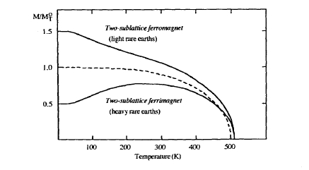
Figure 2.32. Spontaneous magnetization of rare-earth transition-metal intermetallics (schematic). The dashed curve applies to intermetallics containing non-magnetic rare earths such as yttrium.
and
\(T_{\text{RT}} = \frac{2\sqrt{S(S + 1)}\sqrt{J(J + 1)}}{3k_{\text{B}}}\sqrt{z_{\text{RT}}z_{\text{TR}}}(g - 1)\mathcal{J}_{\text{RT}}\). (2.131c)
We see that \(T_{\text{TT}}\) is the Curie temperature of the isolated transition-metal sublattice. It may be estimated from the Curie temperature of isostructural intermetallic compounds containing non-magnetic rare earths such as yttrium. For instance, in the case of \(Tb_{2}Fe_{17}\), where \(T_{\text{C}} = 408\ \text{K}\), \(T_{\text{TT}}\) is estimated as the Curie temperature \(T_{\text{C}} = 317\ \text{K}\) of \(Y_{2}Fe_{17}\).
Often \(T_{\text{TT}} \gg T_{\text{RT}} \gg T_{\text{RR}}\), so that (2.131) simplifies to
\(T_{\text{C}} = T_{\text{TT}}\left(1 + \frac{Gz_{\text{RT}}z_{\text{TR}}\mathcal{J}_{\text{RT}}^{2}}{S(S + 1)z_{\text{TT}}^{2}\mathcal{J}_{\text{TT}}^{2}}\right)\). (2.132)
Both the de Gennes factor \(G = (g - 1)^{2}J(J + 1)\) and the Curie temperature (table 2.9) are largest in the middle of the lanthanide series. A problem with this analysis is that it applies local-moment theory to the itinerant magnetism of 3d electrons in metals, where \(S\) is a non-integral number (section 2.4). In practice, one often uses an effective 3d spin \(S^{*} = m/2\mu_{\text{B}}\).
The temperature dependence of the total magnetization \(M = M_{\text{R}} + M_{\text{T}}\) is obtained numerically from (2.129). The main feature is that the smallness of \(\mathcal{J}_{\text{RT}}\) and \(\mathcal{J}_{\text{RR}}\) leads to a pronounced temperature dependence of the rare-earth sublattice magnetization. Basically, the temperature scale describing the decay of the rare-earth sublattice magnetization is \(\mathcal{J}_{\text{RT}}/k_{\text{B}}\), whereas \(T_{\text{C}}\) is of the order of \(\mathcal{J}_{\text{TT}}/k_{\text{B}}T\). Figure 2.32 shows the schematic temperature dependences of the spontaneous magnetization of two-sublattice ferro- and ferrimagnets. The temperature dependence of the rare-earth sublattice magnetization is closely
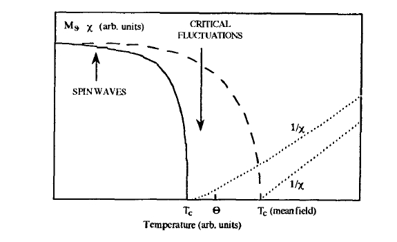
Figure 2.33. Spontaneous ferromagnetic magnetization \(M_{s}\) and inverse Curie–Weiss susceptibility \(1/\chi\) as a function of temperature. The full and dashed curves show the observed and mean-field magnetization curves, respectively.
related to the temperature dependence of the leading rare-earth contribution to the magnetic anisotropy of rare-earth permanent magnets (sections 2.2.4.2 and 3.1.5.2).
Beyond Mean-Field Theory: Advanced Concepts in Magnetism
Although the overall behaviour of the spontaneous magnetization is reasonably well described by the mean-field approximation, there are significant deviations in the low-temperature region and close to the Curie temperature. Figure 2.33 compares the \(M_{s}\) and \(1/\chi\) predictions of the mean-field theories with the behaviour encountered in practice. There are two significant deviations from mean-field theory: at low temperatures the magnetization is overestimated and does not obey the exponential law predicted by the mean-field theory, and there are quantitative and qualitative deviations close to \(T_{\text{C}}\) known as critical behaviour. For example, the mean-field approximation tends to overestimate the Curie temperature.
The reason for the deviations from the mean-field theory is that the assumption of a mean field (molecular field) excludes excitation mechanisms which may be harmful to the spontaneous magnetization. The low-temperature deviations are due to spin waves, also known as magnons, which are a magnetic analogue to elastic lattice vibrations or phonons, whereas the deviations near \(T_{\text{C}}\) are caused by critical fluctuations. Note, for example, that the susceptibility deviates from the Curie–Weiss law \(\chi = C/(T - T_{\text{C}})\) (1.23). Extrapolating the susceptibility well above \(T_{\text{C}}\) to \(1/\chi = 0\) yields the paramagnetic Curie temperature \(\theta_{\text{p}}\). The mean-field theory predicts \(\theta_{\text{p}} = T_{\text{C}}\), but in practice \(\theta_{\text{p}}\) is usually larger than \(T_{\text{C}}\).
A related feature is that mean-field predictions depend on the number \(z\) of interacting neighbours but are independent of the dimensionality \(d\) of the lattice. In fact, there is no ferromagnetic ordering in one-dimensional magnets with short-range interactions, whereas the mean-field theory is qualitatively correct in four or more dimensions20.
Strictly speaking, magnetic order only appears in the thermodynamic limit of infinitely large solids, whereas the mean-field approximation predicts magnetic order in both finite and infinite magnets. Real magnets are a good approximation to the thermodynamic limit.
A pictorial interpretation of the thermodynamic limit is given by the behaviour of a thermally excited ↓ domain in a ↑ ferromagnet. The domain size increases or decreases upon random thermal excitations, but only in finite-size magnets does the thermally activated growth of reversed domains lead, after a possibly very long but always finite time, to magnetic reversal. The statistically averaged, or spontaneous, magnetization of finite-size magnets is therefore zero. In infinite ferromagnets, the reversed domains collapse after a finite time and never lead to the magnetic reversal of the whole magnet. In statistical physics, this phase-space restriction is known as non-ergodic behaviour.
Spin Waves
Experiment shows that the low-temperature spontaneous magnetization of three-dimensional Heisenberg ferromagnets is significantly lower than the mean-field prediction. Far below the Curie temperature, the spontaneous magnetization obeys Bloch's law \(M_{s}(0) - M_{s}(T) \propto T^{3/2}\), whereas the mean-field theory predicts \(M_{s}\) to be constant. This behaviour is caused by spin waves involving the perpendicular spin components \(\hat{S}_{x}\) and \(\hat{S}_{y}\). Classical spin waves are easily understood as being deviations from perfect spin alignment which, due to exchange coupling, propagate through the lattice. On quantization, magnetization of spin waves remains delocalized but always corresponds to an integer number of switched spins.
For simplicity, consider a one-dimensional \(S = 1/2\) Heisenberg spin chain with spacing \(a_{\Delta}\) described by \(\mathcal{H} = -2\mathcal{J}_{0} \sum_{m} \hat{S}(x_{m}) \cdot \hat{S}(x_{m} + a_{\Delta})\) and \(x_{m} = ma_{\Delta}\). Introducing the ladder operators \(\hat{S}_{+,m} = \hat{S}_{x,m} + \text{i}\hat{S}_{y,m}\) and \(\hat{S}_{-,m} = \hat{S}_{x,m} - \text{i}\hat{S}_{y,m}\) the Hamiltonian can be rewritten as
\(\mathcal{H} = -\frac{2\mathcal{J}_{0}}{\hbar^{2}} \sum_{m} (\hat{S}_{z,m} \hat{S}_{z,m + 1} + \frac{1}{2}(\hat{S}_{+,m} \hat{S}_{-,m + 1} + \hat{S}_{-,m} \hat{S}_{+,m + 1}))\). (2.133)
The ladder operators \(\hat{S}_{+,i}\) and \(\hat{S}_{-,i}\) enhance and reduce the \(z\)-projection of the spin \(\hat{S}_{m}\) by \(\mathcal{H}\), respectively, so that products such as \(\hat{S}_{+,m} \hat{S}_{-,m + 1}\) describe the
20 In his seminal paper, Ising (1925) proved that \(T_{\text{C}} = 0\) for the investigated one-dimensional Ising model, as opposed to the non-zero mean-field Curie temperature (2.117). He then concluded that his result can be extended to higher dimensionalities—a crude but highly stimulating misjudgment.
propagation of reversed spins. For instance, the state \(|\uparrow\downarrow\uparrow\rangle\) is transformed into the shifted configuration \(|\uparrow\uparrow\downarrow\rangle\). The spin-wave energies of the one-dimensional Heisenberg chain are obtained by diagonalizing (2.133). It is straightforward to show that the wavefunctions
\(|\psi_{k}\rangle = \frac{1}{N} \sum_{j} e^{ikx_{j}}|j\rangle\) (2.134)
diagonalize equation (2.133) and yield the long-wavelength spin-wave energies \(E_{k} = \mathcal{J}_{0}k^{2}a_{\Delta}^{2}\), where \(a_{\Delta}\) is the distance between the interacting spins21. Since \(E_{k}\) is very low for small \(k\), spin-wave excitations are not restricted to high temperatures.
In more than one dimensions (\(d > 1\)) and for arbitrary spin \(S\), the long-wavelength spin-wave energy is given by
\(E_{k} = D_{2}k^{2}\) (2.135)
where the spin-wave stiffness is given by
\(D_{2} = \frac{z\mathcal{J}_{0}Sa_{\Delta}^{2}}{d}\). (2.136)
This spin-wave stiffness is related to the exchange stiffness (section 3.2.1.1). The quadratic dispersion relation (2.135) is typical of isotropic ferromagnets and leads, in three dimensions, to Bloch's law22
\(M_{s}(0) - M_{s}(T) = 2\zeta(3/2)\mu_{\text{B}} \left(\frac{3k_{\text{B}}T}{4\pi z\mathcal{J}_{0}Sa_{\Delta}^{3}}\right)^{3/2}\). (2.137)
This equation gives a fair description of the spontaneous magnetization up to about \(0.5T_{\text{C}}\). In two dimensions, \(M_{s}(0) - M_{s}(T)\) diverges logarithmically, which indicates the absence of ferromagnetic long-range order. More generally, a theorem due to Mermin and Wagner (1966) states that there is no ferromagnetic long-range order in two-dimensional continuous-symmetry magnets (\(n \geq 2\)). In practice, however, there is always some anisotropy in two-dimensional magnets, so that the Mermin–Wagner theorem does not apply.
A more general spin-wave dispersion relation is \(E_{k} = D_{0}K_{1} + D_{b}k^{b}\), where \(K_{1}\) is the first anisotropy constant and \(b = 1\) and \(b = 2\) for antiferro- and ferromagnets, respectively. The anisotropy term gives rise to an anisotropy gap and leads to the freezing out of the spin waves at very low temperatures. This effect can be used to estimate anisotropy constants. A physical explanation of the spin-wave gap is that the magnetization is captured along the easy axis, so
21 This notation is more general than the use of the cubic lattice parameter \(a\). Note that \(a_{\Delta} = 2R_{\text{nn}}\) and \(a_{\Delta}^{2} = 2a^{2}\) for square, simple cubic (sc), body centred cubic (bcc) and face centred cubic (fcc) lattices; \(z\) is the coordinate number, \(d = 2, 3\) is the lattice dimension.
22 \(\zeta(x) = \sum_{m = 1}^{\infty} m^{-x}\), where \(m = 1, \ldots, \infty\), is the Riemann zeta function; \(\zeta(3/2) \approx 2.612\).
Figure 2.3 . Temperature dependence of the spontaneous magnetization of the square-lattice Ising magnets: mean-field approximation (dashed curve) and Onsager solution (full curve).
that \(M_{s}(T) = M_{s}(0)\) up to a negligibly small exponential correction. Another mechanism not included in (2.136) is the interactions between spin waves, which yield a \(T^{4}\) contribution in addition to Bloch's \(T^{3/2}\) term. Note that spin waves are not restricted to local-moment magnets but also occur in 3d metals. Typical experimental \(D_{2}\) values are \(4.5\), \(8.0\) and \(5.8\ \text{J}\ \text{m}^{2}\) for Fe, Co and Ni, respectively (\(1\ \text{J}\ \text{m}^{2} = 62.4\ \text{meV}\ \text{Å}^{2}\)).
Spin waves not only determine the low-temperature spontaneous magnetization of permanent magnets but are also responsible for the formation of inhomogeneous magnetization states. As we will see in chapter 3, the exchange stiffness \(A\) is proportional to \(D_{2}\) or \(\mathcal{J}_{0}\), which makes it possible to relate micromagnetics to atomic exchange.
The One-dimensional Ising Model
A model exhibiting extreme deviations from the mean-field theory in the critical region close to \(T_{\text{C}}\) is the one-dimensional Ising model. Mean-field theory predicts a spontaneous magnetization (figure 2.28(a)) which, according to (2.117), is non-zero below the mean-field Curie temperature \(2\mathcal{J}_{0}/k_{\text{B}}\). The exact Curie temperature is determined from the zero-field partition function
\(\mathcal{Z} = \sum_{s_{1}=\pm 1} \sum_{s_{2}=\pm 1} \cdots \sum_{s_{N}=\pm 1} \exp\left(\frac{\sum_{i} \mathcal{J}_{0}s_{i}s_{i + 1}}{k_{\text{B}}T}\right)\). (2.138)
This is done by using the microstate variables \(\tau_{i} = s_{i}s_{i + 1} = \pm 1\) rather than \(s_{i} = \pm 1\). Since the transformed Hamiltonian in the exponent of (2.138) does not contain products such as \(\tau_{i}\tau_{i + 1}\), the partition function is that of a paramagnet in \(\tau\) space. As a consequence, there is no finite-temperature phase transition in this model and the exact Curie temperature is zero. Note that this method of
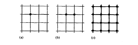
Figure 2.35. Curie-temperature approximations: (a) mean-field approximation, (b) Oguchi approach and (c) exact calculation.
determining \(T_{\text{C}}\) cannot be used in two or more dimensions, since the summation over all products \(\tau_{ik} = s_{i}s_{k} = \pm 1\) creates frustrated spin configurations which do not exist in the original partition function.
Critical Behaviour
The deviations from the mean-field behaviour are particularly pronounced in the vicinity of the critical point \(T = T_{\text{C}}\) and \(H = 0\). Figure 2.34 compares Onsager's exact solution of the square-lattice Ising model
\(\langle s\rangle = (1 - \sinh^{4}(2\mathcal{J}_{0}/k_{\text{B}}T))^{1/8}\) (2.139)
with the mean-field spontaneous magnetization
\(\langle s\rangle = \tanh\frac{4\mathcal{J}_{0}\langle s\rangle}{k_{\text{B}}T}\). (2.140)
A major quantitative effect is the reduction of the Curie temperature compared to the mean-field prediction. A straightforward way to improve the mean-field approximation is by using a cluster calculation. Figure 2.35(b) illustrates the Oguchi method, where an exactly treated two-spin cluster is embedded in the mean field created by the remainder of the lattice. The result of the calculation is
\(k_{\text{B}}T_{\text{C}} = \mathcal{J}_{0}(z - 1)\left(1 + \tanh\frac{\mathcal{J}_{0}}{k_{\text{B}}T_{\text{C}}}\right)\). (2.141)
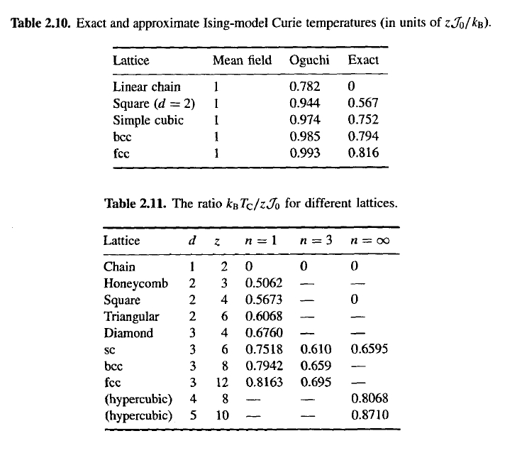
Table 2.10 shows mean-field, Oguchi and exact Curie temperatures for Ising models. We see that the Oguchi improvement on the Curie temperature is small. The ultimate reason for the poor convergence of cluster calculations is that the size of the relevant spin clusters, namely the correlation length, is very large in the vicinity of the critical point.
Numerically calculated numerical Curie temperatures are shown in table 2.11. For some two-dimensional lattices there exist analytical Curie-temperature expressions. For example, the square-lattice Onsager solution yields \(k_{\text{B}}T_{\text{C}} = 2\mathcal{J}_{0}/\ln(1 + \sqrt{2})\).
Critical Exponents
Qualitative differences from the mean-field theory are described in terms of critical exponents. Series expansion of the mean-field expression (2.116) in the vicinity of the critical point yields
\(h = k_{\text{B}}(T - T_{\text{C}})\langle s\rangle + \frac{z\mathcal{J}_{0}}{3}\langle s\rangle^{3}\). (2.142)
This equation of state (materials equation) may equally well be obtained by minimizing the free energy
\(\mathcal{F}_{\text{L}} = \frac{k_{\text{B}}}{2}(T - T_{\text{C}})\langle s\rangle^{2} + \frac{z\mathcal{J}_{0}}{12k_{\text{B}}}\langle s\rangle^{4} - h\langle s\rangle\) (2.143)
with respect to \(\langle s\rangle\). In the phenomenological mean-field or Landau theory, (2.143) is written as \(\mathcal{F}_{\text{L}} = a_{2}\langle s\rangle^{2} + a_{4}\langle s\rangle^{4} - h\langle s\rangle^{23}\).
23 Depending on the physical meaning of the quantities \(a_{2}\), \(a_{4}\), \(\langle s\rangle\) and \(h\), the Landau theory unifies mean-field approaches such as the van der Waals theory in fluid science, Weiss's molecular-field theory in magnetism and the Gorsky-Bragg-Williams approach in physical metallurgy.
Putting \(h = 0\) in (2.142) yields the spontaneous magnetization (order parameter)
\(\langle s\rangle = \sqrt{\frac{3k_{\text{B}}}{z\mathcal{J}_{0}}(T_{\text{C}} - T)^{\beta}}\) (2.144)
where \(\beta = 1/2\). By comparison, the Onsager solution (2.139) yields the critical exponent \(\beta = 1/8\). Note that the difference between the mean-field exponent \(1/2\) and the exact exponent \(1/8\) is clearly visible in figure 2.34: the exact curve is reminiscent of a step function, where \(\beta = 0\).
An important quantity is the correlation function \(\Gamma_{ik} = \Gamma(\mathbf{r}_{i} - \mathbf{r}_{k}) = \langle s_{i}s_{k}\rangle - \langle s_{i}\rangle\langle s_{k}\rangle\) (2.145)
or, in more than one spin dimension, \(\Gamma_{ik} = \langle s_{i} \cdot s_{k}\rangle - \langle s_{i}\rangle \cdot \langle s_{k}\rangle\). As indicated in (2.114), \(\Gamma_{ik}\) describes deviations from the mean-field magnetization (critical fluctuations). Typically, correlations decay as
\(\lim_{R \to \infty} \Gamma(R) \sim e^{-R/\xi}\) (2.146)
where
\(\xi \sim 1/(T - T_{\text{C}})^{\nu}\) (2.147)
is the correlation length. Physically, the correlation length describes the thickness of the interface between \(\uparrow\) and \(\downarrow\) regions (\(T < T_{\text{C}}\)) or the size of ferromagnetically ordered regions (\(T > T_{\text{C}}\)). Note that \(\xi\) must not be confused with the domain-wall width \(\delta\), which reflects macroscopic forces rather than thermal disorder acting on an atomic scale. To calculate the mean-field exponent \(\nu\) we use the Ornstein–Zernike extension of the Landau theory, which amounts to considering the linearized mean-field equation \(k_{\text{B}}T\Gamma_{ij} = h_{i} + \sum_{k} J_{ik}\langle s_{k}\rangle\). Exploiting the relations24 \(\chi_{ik} = \partial\langle s_{i}\rangle/\partial h_{k}\) and \(\Gamma_{ik} = k_{\text{B}}T\chi_{ik}\) yields the matrix representation
\(\Gamma_{ik} = \frac{1}{(\delta_{ik} - J_{ik}/k_{\text{B}}T)}\) (2.148)
where the Kronecker symbol \(\delta_{ik}\) equals one and zero for \(i = k\) and \(i \neq k\), respectively. To obtain the asymptotic behaviour of the correlation function we have to diagonalize the matrix \(J_{ik}\). In the relevant long-wavelength limit, the eigenfunctions are plane waves with the eigenvalues \(\mathcal{J}_{k} = z\mathcal{J}_{0}(1 - a^{2}k^{2}/2d)\). Since \(z\mathcal{J}_{0}\) equals \(k_{\text{B}}T_{\text{C}}\), the Fourier-transformed correlation function is
\(\Gamma(k) = \frac{T}{(T - T_{\text{C}}) + z\mathcal{J}_{0}a^{2}k^{2}/(2k_{\text{B}}d)}\). (2.149)
From this equation, the mean-field exponent \(\nu = 1/2\) is obtained by Fourier transformation. Alternatively we can use dimensional analysis: squared
24 Both equations follow from the functional structure of the partition function. The relation between \(\Gamma_{ik}\) and \(\chi_{ik}\) is known as the fluctuation-dissipation theorem.
wavevectors, including the square of the characteristic wavevector \(k_{0} \approx 1/\xi\), scale as \(T - T_{\text{C}}\) in (2.149).
The zero-field isothermal susceptibility
\(\chi = \frac{\partial\langle s\rangle}{\partial h} = \frac{1}{k_{\text{B}}}(T - T_{\text{C}})^{-\gamma}\) (2.150)
where (2.142) yields \(\gamma = 1\) (the Curie–Weiss law), and the critical isotherm
\(\langle s(T_{\text{C}})\rangle = \left(\frac{3k_{\text{B}}}{z\mathcal{J}_{0}}\right)^{1/3}h^{1/3}\) (2.151)
characterized by the mean-field exponent \(\delta = 3\), shows that \(\beta\), \(\gamma\) and \(\nu\) are not the only critical exponents. Another example is the exponent \(\alpha\), which describes the behaviour of the specific heat near \(T_{\text{C}}\). However, only two exponents are actually independent, since there are only two independent parameters \(z\mathcal{J}_{0}/k_{\text{B}}T\) and \(\mu_{0}\mu_{\text{B}}H/k_{\text{B}}T\) in the partition function. For instance, \(\chi = M/H\) and the definitions of \(\beta\), \(\gamma\) and \(\delta\) may be used to infer the scaling law \(\gamma = \beta(\delta - 1)\). Other scaling laws are \(\alpha = 2 - \nu d\) and \(\alpha + 2\beta + \gamma = 2\).
Universality
It turns out that the critical exponents depend on the lattice dimensionality \(d\) and the number \(n\) of vector-spin components but are independent of lattice structure and the number \(z\) of nearest neighbours. This gives rise to a division of phase transitions into universality classes such as the three-dimensional Heisenberg model and the two-dimensional Ising model. By comparison, Curie-temperature values are non-universal, since they depend, for example, on \(z\). Tables 2.12 and 2.13 show calculated critical exponents for some \(n\)-vector models. Note that the exponents are independent of whether the underlying model is classical or quantum mechanical.
There are general rules for deciding whether the critical exponents deviate from the mean-field predictions. On the one hand, mean-field exponents are exact in more than four dimensions. The dimensionality four is a borderline case, where there are often logarithmic corrections to the mean-field
exponents. On the other hand, long-range interactions extend the validity of the mean-field theory to less than four dimensions25. Note, for example, that infinite Ising chains having \(\mathcal{J}_{ik} = \mathcal{J}'\) for all inter-atomic distances \(|\mathbf{r}_{i} - \mathbf{r}_{k}|\) may not be distinguished from three- or four-dimensional infinite-range Ising magnets.
In the practically important limit of finite-range or short-range interactions, there are various methods of determining critical exponents. Experimentally, double-logarithmic data plots are used, while computer simulations are a powerful numerical method. In some cases it has been possible to obtain analytical results. Examples are the Ising model in one and two dimensions and the spherical model in less than four dimensions, where \(\beta = 1/2\), \(\gamma = 2/(d - 2)\), \(\delta = (d + 2)/(d - 2)\) and \(\nu = 1/(d - 2)\). A straightforward method is the analysis of series expansions of the partition function.
A famous way of calculating critical exponents is renormalization-group analysis, where the properties of the original lattice are compared with those of a lattice expanded by a scaling factor (Wilson 1983). It turns out that iterative scaling conserves the physics of the magnetic if the correlation length is much larger than the range of interaction (see appendix A4.4). This makes it possible to deduce critical exponents from renormalization-group equations. Close to the critical dimension four, that is for \(d = 4 - \varepsilon\), perturbation theory yields the critical exponents \(\gamma = 1 + 0.5\varepsilon(n + 2)/(n + 8)\), \(\delta = 3 + \varepsilon\), \(\beta = 1/2 - 1.5\varepsilon/(n + 8)\) and \(\nu = 1/2 + 0.25\varepsilon(n + 2)/(n + 8)\).
Very close to \(T_{\text{C}}\) the magnetic anisotropy gives rise to deviations from Heisenberg behaviour. The same is true of magnetoelastic interactions, which are small but long range. However, since critical phenomena refer to the immediate vicinity of \(T_{\text{C}}\) they are of secondary importance in permanent magnetism: the mean-field approximation is used nearly exclusively to describe the temperature dependence of the magnetization.
25 Examples are superconductors, where the long-range character of the problem is associated with the formation of Cooper pairs, and gases in metals, where the distribution of the gas atoms is governed by long-range elastic interactions.