
2.2 Magnetic ions
Magnetic lons: The Building Blocks of Magnetism
Since solid-state magnetism is caused by electrons in the partly filled inner shells of rare-earth and transition-metal atoms, the properties of ions such as Fe2+ and Nd3+ are of great importance. The point is that the electrostatic interaction between degenerate electrons is very effective in creating a magnetic moment, and to some extent the ionic properties survive the incorporation into metallic and non-metallic solids. This applies particularly to the rare-earth 4f shells, where the atomic environment acts as a small perturbation. By comparison, the comparatively large radius of iron-series 3d shells (figure 2.17) leads to the suppression (quenching) of the orbital moment in both insulators and metals. The quenching of the orbital moment has two main consequences: (i) the magnetic moment of 3d electrons is obtained by spin counting and (ii) the anisotropy contribution of 3d electrons is comparatively small. Furthermore, inter-atomic hopping leads to the delocalization of 3d electrons in metals. However, even in the metallic limit the 3d electrons keep some ionic character, which is seen for example from the 3d charge density. In this section we review the properties of magnetic ions without reference to their crystalline environment.
Atomic Wavefunctions and Their Role in Magnetism
To discuss ionic properties one has to start from atomic one-electron wavefunctions, such as hydrogen-like orbitals, which may then be used to construct approximate many-electron wavefunctions. There are two types of hydrogen-like wavefunctions: quenched (real) wavefunctions and unquenched (complex) wavefunctions.
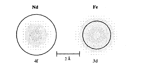
Figure 2.17. Electron density of partially filled shells in rare-earth and transition-metal ions (schematic). The solid circles indicate the metallic radii.
Schrödinger Equation
Consider a single electron moving in the electrostatic central potential created by a positive nuclear charge \(Q = Ze\), so that (2.14) becomes
\(E_{\mu}\psi_{\mu} = -\frac{h^{2}}{2m_{e}}\nabla^{2}\psi_{\mu} - \frac{Ze^{2}}{4\pi\epsilon_{0}r}\psi_{\mu}\). (2.73a)
It is instructive here to express energies in terms of the Bohr radius \(a_{0} = 4\pi\epsilon_{0}\hbar^{2}/m_{e}e^{2} \approx 52.9 \text{ pm }(0.529 \text{ Å})\) and Sommerfeld's fine-structure constant \(\alpha = e^{2}/4\pi\epsilon_{0}\hbar c \approx 1/137\)
\(E_{\mu}\psi_{\mu} = -\frac{\alpha^{2}a_{0}^{2}m_{e}c^{2}}{2}\nabla^{2}\psi_{\mu} - \frac{Z\alpha^{2}a_{0}m_{e}c^{2}}{r}\psi_{\mu}\). (2.73b)
This equation yields one-electron orbitals characterized by three quantum numbers: the principal quantum number \(n\), the azimuthal or angular quantum number \(l\) and the magnetic quantum number \(m_{l}\).
The principal quantum number \(n\) defines electron shells, which divide into subshells \(0 \leq l \leq n - 1\) characterized by an orbital quantum number \(l\). For historical reasons the orbital quantum states are written as s, p, d and f rather than 1, 2, 3 and 4. Since each subshell contains \(2l + 1\) magnetic quantum states \(m_{l} = -l, \ldots, 0, \ldots, l\) and each orbital characterized by the three quantum numbers \(n\), \(l\) and \(m_{l}\) can accommodate a pair of \(\uparrow\) and \(\downarrow\) electrons, there are at most \(2n^{2}\) electrons in the \(n\)th shell. For example, the \(l = 2\) subshell of the third shell is denoted by 3d, contains five states \(m_{l} = 0, \pm 1, \pm 2\) and is occupied by up to 10 electrons. Similarly, the 3s and 3p subshells contain two and six electrons, respectively, so that there are altogether \(2 \times 3^{2} = 18\) orbitals in the third shell.
It turns out that the eigenfunctions of (2.73) are \(2n^{2}\)-fold degenerate, that is the \(2n^{2}\) states of the \(n\)th shell have the same energy
\(E_{n} = -\frac{1}{n^{2}}\frac{1}{2}m_{e}(Z\alpha c)^{2}\). (2.74)
The degeneracy with respect to the magnetic quantum number \(m_{l}\) arises from the sphericity of the Coulomb potential and is removed by an external magnetic field. By comparison, the degeneracy with respect to \(l\) is a specific feature of the \(1/r\) radial dependence of the hydrogen-like potential. In real atoms, the Coulomb interaction with electrons in other shells and subshells yields deviations from the \(1/r\) potential and eliminates the subshell degeneracy.
Hydrogen-like Wavefunctions
In polar coordinates the complex hydrogen-like wavefunctions are (see appendix A2)
\(\psi_{nlm}(r,\theta,\phi) = R_{nl}(r)Y_{l}^{m}(\phi,\theta)\). (2.75)
Here both \(R_{nl}\) and \(Y_{l}^{m}\) are orthogonal and normalized:
\(\int R_{nl}R_{n'l'}(r)r^{2} dr = \delta_{nn'}\delta_{ll'}\)
and
\(\int Y_{l}^{*m}(\phi,\theta)Y_{l'}^{m'}(\phi,\theta) \sin\theta d\theta d\phi = \delta_{ll'}\delta_{mm'}\).
For example, the 3d wavefunctions characterized by \(\ell = 2\) and \(m_{l} = \pm 2\) are
\(\psi(r,\theta,\phi) = \sqrt{\frac{15}{32\pi}}R_{3d}(r)\sin^{2}\theta e^{\pm 2i\phi}\). (2.76)
Besides the complex 3d wavefunctions \(|0\rangle\), \(|\pm 1\rangle\) and \(|\pm 2\rangle\) there exists a set of five real wavefunctions \(|\mu\rangle\) commonly denoted by \(|xy\rangle\), \(|yz\rangle\), \(|zx\rangle\), \(|x^{2} - y^{2}\rangle\) and \(|z^{2}\rangle\). For example,
\(|xy\rangle = \sqrt{\frac{15}{16\pi}}R_{3d}(r)\sin^{2}\theta \sin 2\phi\) (2.77a)
and
\(|x^{2} - y^{2}\rangle = \sqrt{\frac{15}{16\pi}}R_{3d}(r)\sin^{2}\theta \cos 2\phi\). (2.77b)
Figure 2.18 shows the angular dependence of the real 3d wavefunctions. Note that
\(|\pm 2\rangle = \frac{1}{\sqrt{2}}|x^{2} - y^{2}\rangle \pm \frac{i}{\sqrt{2}}|xy\rangle\). (2.78)
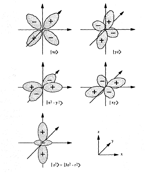
Figure 2.18. Real atomic 3d wavefunctions (schematic).
A similar relation exists between the \(m_{l} = 1\) orbitals \(|xz\rangle\), \(|yz\rangle\) and \(|\pm 1\rangle\), whereas \(|0\rangle = |z^{2}\rangle\).
Due to their completeness and orthonormality, both sets of atomic wavefunctions can be used to describe atomic 3d magnetism. The difference between real and complex wavefunctions is seen from the quantum-mechanical orbital-momentum average
\(\langle l_{z}\rangle = \frac{1}{2\pi} \int \psi^{*}(\phi)(-i\hbar\partial /\partial\phi)\psi(\phi) d\phi\). (2.79)
It is easy to show that complex and real wavefunctions yield \(\langle l_{z}\rangle = m_{l}\hbar\) and \(\langle l_{z}\rangle = 0\), respectively. In 3d magnets, the orbital momentum is normally suppressed, which is known as quenching (section 2.2.2.4).
The largely spherical potentials encountered in atomic physics make it possible to start from hydrogen-like wavefunctions except that subshell energies increase with \(l\) so that, for example, \(2p\) electrons have higher energies than \(2s\) electrons. This rule gives rise to ground-state electron configurations such as \(1s^{2}2s^{2}2p^{6}3s^{1}\) for sodium, where the superscripts denote the number of electrons in the subshells.
Apart from a minor diamagnetic correction, completely filled inner electron shells (noble-gas shells) are magnetically inert and do not need to be considered in the present context8. The noble-gas electron cores of main-group atoms are surrounded by chemically active valence electrons, but chemical interaction tends to yield magnetically inert \(\uparrow \downarrow\) occupancies. For example, atomic nitrogen has the electron configuration \([He]2s^{2}2p^{3}\) and contains unpaired \(2p\) electrons, but in molecular nitrogen \((N_{2})\) all electrons are paired. In chapter 5 we will see how main-group elements are used to modify permanent magnetic properties (H, C, N) or stabilize desired crystal structures (B, Sr, Ba).
Solid-state magnetism originates from unpaired electrons in the partly filled inner shells of transition metals. Examples are Fe and Nd atoms, which have the respective electron structures \([Ar]3d^{6}4s^{2}\) and \([Xe]4f^{4}6s^{2}\). According to the quantum numbers of the partly filled shells (table 1.2), transition metals are classified as iron-series metals (3d elements), palladium series metals (4d elements), platinum series metals (5d elements), rare earths (4f elements) and actinides (5f elements). A feature of the partly filled inner shells is their comparatively small radius (figure 2.17). This reduces the interaction with the atomic environment and makes it possible to treat the atoms as magnetic ions.
Rare-earth atoms in metals and insulators tend to form tripositive ions such as \(Nd^{3+}\), whereas elements of the iron series have two or more possible oxidation states. As a rule, oxides of early 3d elements are particularly stable if they contain \(T^{3+}\) or \(T^{4+}\) ions, whereas the late 3d elements are more likely to form \(T^{2+}\) or \(T^{3+}\) ions in oxides and halides. Examples are \(Fe^{2+}\) (ferrous iron, \(3d^{6}\)) and \(Fe^{3+}\) (ferric iron, \(3d^{5}\)). The applicability of the ionic picture to metallic 3d atoms is very limited, because the strong inter-atomic hopping modifies the electronic wavefunctions. As a crude approximation, one may think of late 3d atoms in metals as \(T^{1+}\) ions, with one 4s conduction electron.
Although many permanent magnets of practical importance are based on 3d and 4f elements, there exist materials such as PdFe and PtCo, where the comparatively large spin-orbit coupling of 4d or 5d elements is exploited (section 5.2). Spin-orbit coupling is even greater in actinide compounds such as US, but most other intrinsic magnetic properties of actinide compounds are poor. Ions such as \(La^{3+} (4f^{0})\), \(Lu^{3+} (4f^{14})\) and \(Y^{3+} (4d^{0})\) may be regarded as magnetically inert.
as non-magnetic rare ions, since empty and completely filled subshells are magnetically inert.
lonic Moments: The Key to Magnetic Behavior
Electrons in ions are not independent but interact electrostatically, so that the properties of the individual electrons do not just superpose to yield the ionic behaviour. A good example is the total angular momentum \( \vec{J} \) of the ion, which obeys \( \hat{L}_{z}|\Psi\rangle = \hbar L_{z}|\Psi\rangle \) and \( \hat{J}^{2}|\Psi\rangle = \hbar^{2}J(J + 1)|\Psi\rangle \).
Basic Features
Rare-earth 4f-shell radii and ionic radii are around 50 pm and 100 pm (0.5 Å and 1.00 Å), respectively, whereas the metallic radii of the rare earths are about 180 pm (1.80 Å). This nearly complete isolation of the 4f electrons from the crystal environment ensures well conserved ionic properties and we can assume that intra-atomic Coulomb and exchange contributions dominate. The moderate strength of the rare-earth spin-orbit coupling means that the total angular momentum of the ion is the sum or difference of the ionic spin and orbital moments. This mechanism is called \( L - S \) or Russell-Saunders coupling, as opposed to the \( j - j \) coupling important in inner shells of very heavy elements, where the spin-orbit interaction dismantles the ionic spin and orbital momenta. Inter-atomic exchange and crystal-field interactions are small perturbations in the present context9. As a consequence, the ground states of rare-earth ions obey Hund's rules known from quantum chemistry and spectroscopy. In 3d magnets, Hund's rules are only partly satisfied.
Hund's Rules
The electronic structure of incompletely filled subshells involves intra-atomic exchange and spin-orbit coupling. Although the ground state of incompletely filled subshells may be determined by numerical calculations, it is more convenient to use semi-empirical rules (Hund 1925).
(i) Subject to the Pauli principle, the total spin \( S = |\sum_{i} s_{zi}| \) is maximized.
(ii) Subject to the Pauli principle and the first rule, the total orbital momentum \( L = |\sum_{i} l_{zi}| \) is maximized.
(iii) \( L \) and \( S \) couple parallel, \( J = |L + S|\), in more-than-half-filled shells and couple antiparallel, \( J = |L - S|\), in less-than-half-filled shells.
Generally, the first two rules are supported by larger energy differences than the third rule, which reflects the comparatively weak spin-orbit coupling. Tables 2.4 and 2.5 show the ground states of Hund's rule of free 3d and 4f ions.
9 In the case of rare-earth atoms, these contributions affect anisotropy (section 3.1.3) and magnetic order (section 2.2.4) but leave the magnetic moment unchanged.
Table 2.4. Ground states of 3d ions. The boxes indicate the filling of the 3d shell. In solids, the orbital angular momentum is usually quenched, \(g \approx 2\) and \(p_{eff}\) is the spin-only effective moment.
| +2 | +1 | 0 | -1 | -2 | S | L | J | g | gJ | peff | |
|---|---|---|---|---|---|---|---|---|---|---|---|
| 3d1 Ti3+, V4+ | ↓ | — | — | — | — | 1/2 | 2 | 3/2 | 4/5 | 6/5 | 1.73 |
| 3d2 V3+, Cr4+ | ↓ | ↓ | — | — | — | 1 | 3 | 2 | 2/3 | 4/3 | 2.83 |
| 3d3 Cr3+, Mn4+ | ↓ | ↓ | ↓ | — | — | 3/2 | 3 | 3/2 | 2/5 | 3/5 | 3.87 |
| 3d4 Cr2+, Mn3+ | ↓ | ↓ | ↓ | ↓ | — | 2 | 2 | — | 0 | 0 | 4.90 |
| 3d5 Mn2+, Fe3+ | ↓ | ↓ | ↓ | ↓ | ↓ | 5/2 | 0 | 5/2 | 2 | 5 | 5.92 |
| 3d6 Fe2+, Co3+ | ↑↓ | ↑ | ↑ | ↑ | ↑ | 2 | 2 | 4 | 3/2 | 6 | 4.90 |
| 3d7 Co2+, Ni3+ | ↑↓ | ↑↓ | ↑ | ↑ | ↑ | 3/2 | 3 | 9/2 | 4/3 | 6 | 3.87 |
| 3d8 Ni2+, Co+ | ↑↓ | ↑↓ | ↑↓ | ↑ | ↑ | 1 | 3 | 4 | 5/4 | 5 | 2.83 |
| 3d9 Cu2+, Ni+ | ↑↓ | ↑↓ | ↑↓ | ↑↓ | ↑ | 1/2 | 2 | 5/2 | 6/5 | 3 | 1.73 |
Table 2.5. Ground states of 4f ions . The boxes indicate the filling of the f shell.
| +3 | +2 | +1 | 0 | -1 | -2 | -3 | S | L | J | g | gJ | \(p_{eff}\) | |
|---|---|---|---|---|---|---|---|---|---|---|---|---|---|
| 4f1 Ce3+ | ↓ | — | — | — | — | — | — | 1/2 | 3 | 5/2 | 6/7 | 15/7 | 2.54 |
| 4f2 Pr3+ | ↓ | ↓ | — | — | — | — | — | 1 | 5 | 4 | 4/5 | 16/5 | 3.58 |
| 4f3 Nd3+ | ↓ | ↓ | ↓ | — | — | — | — | 3/2 | 6 | 9/2 | 8/11 | 36/11 | 3.62 |
| 4f4 Pm3+ | ↓ | ↓ | ↓ | ↓ | — | — | — | 2 | 6 | 4 | 3/5 | 12/5 | 2.68 |
| 4f5 Sm3+ | ↓ | ↓ | ↓ | ↓ | ↓ | — | — | 5/2 | 5 | 5/2 | 2/7 | 5/7 | 0.85 |
| 4f6 Eu3+ | ↓ | ↓ | ↓ | ↓ | ↓ | ↓ | — | 3 | 3 | 0 | — | 0 | — |
| 4f7 Gd3+ | ↓ | ↓ | ↓ | ↓ | ↓ | ↓ | ↓ | 7/2 | 0 | 7/2 | 2 | 7 | 7.94 |
| 4f8 Tb3+ | ↑↓ | ↑ | ↑ | ↑ | ↑ | ↑ | ↑ | 3 | 3 | 6 | 3/2 | 9 | 9.72 |
| 4f9 Dy3+ | ↑↓ | ↑↓ | ↑ | ↑ | ↑ | ↑ | ↑ | 5/2 | 5 | 15/2 | 4/3 | 10 | 10.65 |
| 4f10 Ho3+ | ↑↓ | ↑↓ | ↑↓ | ↑ | ↑ | ↑ | ↑ | 2 | 6 | 8 | 5/4 | 10 | 10.61 |
| 4f11 Er3+ | ↑↓ | ↑↓ | ↑↓ | ↑↓ | ↑ | ↑ | ↑ | 3/2 | 6 | 15/2 | 6/5 | 9 | 9.58 |
| 4f12 Tm3+ | ↑↓ | ↑↓ | ↑↓ | ↑↓ | ↑↓ | ↑ | ↑ | 1 | 5 | 6 | 7/6 | 7 | 7.56 |
| 4f13 Yb3+ | ↑↓ | ↑↓ | ↑↓ | ↑↓ | ↑↓ | ↑↓ | ↑ | 1/2 | 3 | 7/2 | 8/7 | 4 | 4.54 |
Ionic states are usually labelled with the spectroscopic Russell-Saunders notation. Levels characterized by well defined ionic quantum numbers \(L\) and \(S\)
form a term denoted by \(^{2S + 1}L\). Here the prefix \(2S + 1\) is the spin multiplicity and the orbital momentum \(L\) is written as S, P, D,.... analogous to the one-electron notation s, p, d,.... For example, the term symbol \(^{2}\text{D}\) means \(L = 2\) and \(S = 1/2\). Spin-orbit coupling causes ionic terms to split into multiplets denoted by \(^{2S + 1}L_{J}\), where \(|L - S| \leq J \leq |L + S|\). For instance, the \(^{2}\text{P}\) term splits into a \(^{2}\text{P}_{1/2}\) doublet and a \(^{2}\text{P}_{3/2}\) quartet. According to Hund's third rule, the ground-state multiplet obeys \(J = |L \pm S|\). It turns out that excited multiplets of most rare-earth ions have fairly high energies and can be neglected. Notable exceptions are Eu3+ and Sm3+, where the energy splitting between the lowest-lying multiplets is of order 0.1 eV so that thermal and magnetic perturbations may be important. Finally, the remaining \((2J + 1)\)-fold intra-multiplet degeneracy is removed by interactions such as Zeeman coupling and inter-atomic exchange.
Zeeman Splitting and The Landé Factor
The magnetic moment of an ion is determined by the intra-multiplet splitting in an external magnetic field \( \mathbf{H} = H e_{z} \) (figure 2.19), and by analogy with the Zeeman term in (2.35) we have to consider the ionic operator \( \hat{\mathbf{L}} + 2\hat{\mathbf{S}} \). The relevant quantum-mechanical average \( \langle\Psi|(\hat{L}_{z} + 2\hat{S}_{z})|\Psi\rangle \) depends on the functional structure of the wavefunction. In the present context, \( L \), \( S \), \( J \) and \( J_{z} \) are known, and the wavefunction has the functional structure \( |\Psi\rangle = |LSJ J_{z}\rangle \). It would be more convenient to use the wavefunction \( |\Psi'\rangle = |L L_{z} S S_{z}\rangle \), leading to \( \langle\Psi'|(\hat{L}_{z} + 2\hat{S}_{z})|\Psi'\rangle = L_{z} + 2S_{z} \), but \( L_{z} \) and \( S_{z} \) are ill defined in the context of the magnetism of Hund's rules. The reason is that \( \hat{\mathbf{L}} \) and \( \hat{\mathbf{S}} \) are not necessarily parallel and the calculation of \( \langle\Psi|\hat{S}_{z}|\Psi\rangle \) involves the projection of \( \hat{\mathbf{S}} \) onto \( \hat{\mathbf{J}} \).
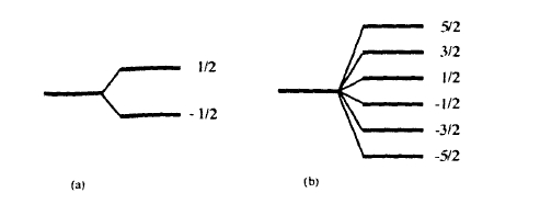
Figure 2.19. Intramultiplet splitting (Zeeman splitting) of multiplets: (a) single electron (S = 1/2, L = 0, J = 1/2) and (b) Sm3+ (S = 5, L = 5/2, J = 5/2). The levels are labelled by \(J_{z}\).
To calculate the level splitting we write
\(\hat{\mathbf{L}} + 2\hat{\mathbf{S}} = \hat{\mathbf{J}} + \hat{\mathbf{S}} = g\hat{\mathbf{J}}\) (2.80)
where \(g\) is the Landé factor. The \(g\) factor is the ratio of the magnetic moment of the ion in Bohr magnetons to the angular momentum in units of \(\hbar\). The projection
\(g\hat{\mathbf{J}}^{2} = \hat{\mathbf{J}}^{2} + \hat{\mathbf{S}} \cdot \hat{\mathbf{J}}\) transforms the vector expression (2.80) into a scalar equation but contains the inconvenient product \(\hat{\mathbf{S}} \cdot \hat{\mathbf{J}} = \hat{\mathbf{S}} \cdot \hat{\mathbf{L}} + \hat{\mathbf{S}}^{2}\). To remove the mixed terms we exploit the identity \(\hat{\mathbf{J}}^{2} = \hat{\mathbf{S}}^{2} + 2\hat{\mathbf{S}} \cdot \hat{\mathbf{L}} + \hat{\mathbf{L}}^{2}\) and obtain with \(\langle\Psi|\hat{L}^{2}|\Psi\rangle = \hbar^{2}L(L + 1)\), \(\langle\Psi|\hat{S}^{2}|\Psi\rangle = \hbar^{2}S(S + 1)\) and \(\langle\Psi|\hat{J}^{2}|\Psi\rangle = \hbar^{2}J(J + 1)\) the result
\(g = \frac{3}{2} + \frac{S(S + 1) - L(L + 1)}{2J(J + 1)}\). (2.81)
When only the spin is relevant, as is the case for exchange interaction, then one has to use the projection \(\langle S_{z}\rangle = (g - 1)\langle J_{z}\rangle\) (section 2.3). Note that \(g = 1 - S/(J + 1)\) and \(g = 1 + S/J\) for the first and second halves of the lanthanide series, respectively (table 2.5).
Quenching
Experiment shows that 3d ions in solids have \(L \approx 0\), \(J \approx S\) and \(g \approx 2\), which disagrees with the predictions of Hund's rules. The elimination of the orbital moment \(L_{z}\) by the crystal field is known as quenching of the orbital angular momentum. As a consequence, the moment of 3d atoms, measured in \(\mu_{B}\), equals the number of unpaired electrons. For instance, ferric iron (Fe3+) has a 3d5 configuration, i.e. a half-filled shell, and the five \(\uparrow\) electrons yield \(m = 5\ \mu_{B}\). In ferrous iron (Fe2+) there are six 3d electrons per ion. Again, five electrons occupy \(\uparrow\) states, but the sixth electron has to occupy a \(\downarrow\) orbital, so that the total moment is only \(m = 4\ \mu_{B}\). This rule makes it easy to estimate the moment of 3d oxides by adding all atomic contributions. For example, magnetite Fe3O4 = FeO.Fe2O3 contains two Fe3+ ions with antiparallel ionic moments and one Fe2+ ion. This yields the prediction of \(4\ \mu_{B}\) per formula unit, which is very close to the observed value \(4.1\ \mu_{B}\). In 3d metals, where the number of 3d electrons per atom is non-integral, the orbital-moment contribution is only of the order of \(0.1\ \mu_{B}\).
In section 2.2.1.2 we have seen that orbital angular momentum is associated with the real or complex character of the wavefunctions. It turns out that the competition between the spin-orbit coupling and the crystal-field interaction decides whether the wavefunctions are real or complex (table 2.6). Real wavefunctions can be interpreted as standing waves and are characterized by a strong azimuthal variation of the electronic charge density \(-e\psi^{*}(\phi)\psi(\phi)\). This enables them to adapt their charge density to the crystal field of the lattice (figure 2.20(a)). A good example are ionic d wavefunctions in sites of cubic symmetry with an inversion centre, where in the absence of spin-orbit coupling \(|xy\rangle\), \(|yz\rangle\) and \(|zx\rangle\) form a degenerate set, denoted \(t_{2g}\), and \(|x^{2} - y^{2}\rangle\) and \(|z^{2}\rangle\) form another degenerate set, denoted \(e_{g}\) (figure 2.18). By contrast, complex wavefunctions can be interpreted as running waves characterized by a comparatively smooth charge distribution (figure 2.20(b)). They are electrostatically unfavourable but benefit from spin-orbit coupling.
The small radius of the rare-earth 4f shells leads to a comparatively strong spin-orbit coupling, whereas the crystal field is largely screened by conduction
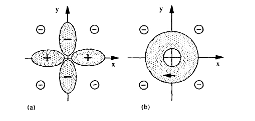
Figure 2.20. Real (a) and complex (b) wavefunctions in a crystal field created by four negative charges. The crystal-field interaction and spin-orbit coupling favour (a) and (b), respectively.
Table 2.6. Quenched and unquenched wavefunctions.
| Quenched limit | Unquenched limit | |
|---|---|---|
| Wavefunction | Real | Complex |
| Character | Standing waves | Running waves |
| Landé factor | \(g = 2\) | \(g \neq 2\) |
| Orbital moment | Zero | Non-zero |
| Spin-orbit coupling | Small | Large |
| Energy in the crystal field | Low | High |
| Realized in | 3d ions | 4f ions |
electrons. For this reason, complex wavefunctions are energetically more favourable than real wavefunctions and 4f moments remain unquenched. The opposite is true for 3d atoms in metals and insulators: the strong crystal field acting on iron-series 3d atoms and the comparatively low spin–orbit coupling lead to a nearly complete quenching of 3d orbital moments.
Charge Distribution in Magnetic lons: what lt Means
The generally aspherical charge distribution of the incompletely filled inner shells is of great importance, because the shells interact electrostatically with the anisotropic crystal field. Transmitted by spin–orbit coupling, this crystal-field interaction gives rise to magnetocrystalline anisotropy (sections 3.1.3 and 5.3.2.1). This refers, in particular, to the 4f anisotropy in rare-earth permanent magnets, where the comparatively strong 4f spin–orbit coupling assures well defined ionic charge distributions. By comparison, the charge distribution of 3d atoms is strongly crystal-field dependent and cannot be interpreted as a purely ionic property.
Multipole Moments
The strong rare-earth spin-orbit interaction means that the symmetry axis of the 4f charge cloud is parallel to the magnetization. We suppose in this section that the magnetization is parallel to \(e_{z}\). By expanding the 4f charge distribution in spherical harmonics it can be shown that the lowest-order aspherical contribution to the 4f charge density is
\(n_{4f}(r)=\frac{5Q_{2}}{16\pi(r^{2})_{4f}}(3\cos^{2}\theta - 1)R_{4f}(r)\). (2.82)
Here \(r = r(\sin\theta\cos\phi e_{x} + \sin\theta\cos\phi e_{y} + \cos\theta e_{z})\) and \(R_{4f}(r)\) is the radial part of the 4f wavefunction, so that \(\int R_{4f}(r)^{*}r^{2}R_{4f}(r) dr = (r^{2})_{4f}\). The electrostatic quadrupole moment of the ion10 is given by
\(Q_{2}=\int n_{4f}(r)(3\cos^{2}\theta - 1)r^{2} dr\). (2.83)
The sign of \(Q_{2}\) decides whether the 4f electron cloud is prolate (\(Q_{2} > 0\)) or oblate (\(Q_{2} < 0\)). Similarly, hexadecapole and 64-pole moments are defined as
\(Q_{4}=\int n_{4f}(r)(35\cos^{4}\theta - 30\cos^{2}\theta + 5)r^{4} dr\) (2.84)
and
\(Q_{6}=\int n_{4f}(r')(231\cos^{6}\theta - 315\cos^{4}\theta + 105\cos^{2}\theta - 5)r^{6} dr\) (2.85)
respectively. Higher-order moments decide, for instance, whether a prolate charge distribution resembles a bone (\(Q_{4} < 0\)) or a snake which has just eaten a rabbit (\(Q_{4} > 0\)). The rotational symmetry of the 4f charge distribution is associated with the absence of quenching.
The calculation of the rare-earth multipole moments is reminiscent of the calculation of the Landé factor (2.81) although somewhat more complicated. A trivial exception are ions with filled or half-filled shells, such as Gd3+, which are spherical and do not contribute to the anisotropy. On the other hand, from the angular dependence of the 4f wavefunctions it follows that odd multipole moments such as the dipole moment \(Q_{1}\) and those higher than the 64-pole moments are zero. Only in a few cases is it possible to represent the multipole moments \(Q_{m}\) in terms of closed expressions. For example, the \(J = J_{z}\) ground-state quadrupole moments of the heavy rare-earth ions with \(n4f\) electrons (\(n \geq 7\)) are given by
\(Q_{2}=-\frac{1}{45}(14 - n)(7 - n)(21 - 2n)(r^{2})_{4f}\). (2.86)
Note, furthermore, that \(Q_{m}=0\) for \(J < m/2\), which implies that the 64-pole moments vanish for the \(J = 5/2\) ground states of Ce3+ and Sm3+.
10 The ionic multipole moments should not be confused with the quadrupole moments of the nuclei.
Table 2.7. Shapes of tripositive rare-earth ions in their ground states of the Hund's rule.
(Based on data given by Freeman and Watson (1962) and Hutchings (1964). Note the common use of \(a_{0} = 59.29\ pm (0.5929\ Å)\) as a unit here.)
| \(n\) | \(J\) | \(Q_{2}/(r^{2})_{4f}\) | \(Q_{4}/(r^{4})_{4f}\) | \(Q_{6}/(r^{6})_{4f}\) | \(\frac{Q_{2}}{(a_{0}^{2})}\) | \(\frac{Q_{4}}{(a_{0}^{4})}\) | \(\frac{Q_{6}}{(a_{0}^{6})}\) | |
|---|---|---|---|---|---|---|---|---|
| Ce | 1 | 5/2 | -4/7 | 0.3810 | 0 | -0.686 | 1.316 | 0 |
| Pr | 2 | 4 | -1456/2475 | -0.6171 | 0.3074 | -0.639 | -1.314 | 4.834 |
| Nd | 3 | 9/2 | -28/121 | -0.4402 | -0.5744 | -0.232 | -1.057 | -7.120 |
| Pm | 4 | 4 | 392/1815 | 0.3423 | 0.4814 | 0.202 | 0.729 | 3.186 |
| Sm | 5 | 5/2 | 26/63 | 0.1501 | 0 | 0.364 | 0.285 | 0 |
| Tb | 8 | 6 | -2/3 | 0.7273 | -0.1865 | -0.505 | 1.047 | -1.082 |
| Dy | 9 | 15/2 | -2/3 | -0.9697 | 0.9324 | -0.484 | -1.282 | 4.757 |
| Ho | 10 | 8 | -4/15 | -0.7273 | -1.8648 | -0.185 | -0.887 | -8.392 |
| Er | 11 | 15/2 | 4/15 | 0.7273 | 1.8648 | 0.178 | 0.819 | 7.418 |
| Tm | 12 | 6 | 2/3 | 0.9697 | -0.9324 | 0.427 | 0.999 | -4.201 |
| Yb | 13 | 7/2 | 2/3 | -0.7273 | 0.1865 | 0.409 | -0.698 | 0.579 |
Equivalent Operators
A method to determine the multipole moments is to use equivalent operators \(\hat{O}_{\pi}^{m}\) (Hutchings 1964) such as
\(\hat{O}_{2}^{0}=\frac{1}{\hbar^{2}}(3\hat{J}_{z}^{2}-\hat{J}^{2})\). (2.87)
These are discussed in section 3.1.3.4. The involvement of angular-momentum operators makes it possible to use calculational tools such as the Wigner–Eckart theorem (Ashcroft and Mermin 1976) and yields for \(J_{z}=J\)
\(Q_{2}=\theta_{2}\langle r^{2}\rangle_{4f}(2J^{2}-J)\) (2.88)
\(Q_{4}=\theta_{4}\langle r^{4}\rangle_{4f}(8J^{4}-24J^{3}+22J^{2}-6J)\) (2.89)
and
\(Q_{6}=\theta_{6}\langle r^{6}\rangle_{4f}(16J^{6}-120J^{5}+340J^{4}-450J^{3}+274J^{2}-60J)\) (2.90)
where \(\theta_{2}\), \(\theta_{4}\) and \(\theta_{6}\) are the second-, fourth- and sixth-order Stevens coefficients, respectively11.
Table 2.7 shows 4f multipole data. For example, \(Q_{2} = -1360\ pm^{2}\) \((-0.136\ Å^{2})\) for the Dy3+ ground state, the negative sign indicating that the
11 An alternative notation is \(\alpha_{J}=\theta_{2}\), \(\beta_{J}=\theta_{4}\) and \(\gamma_{J}=\theta_{6}\).
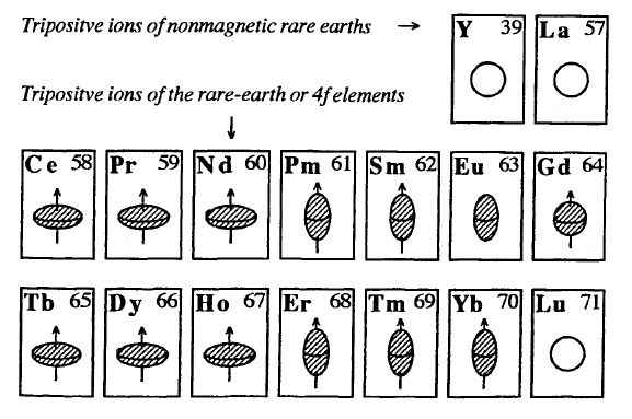
Figure 2.21. Shapes of 4f electron clouds of rare-earth ions (schematic). Empty circles indicate non-magnetic ions. The ionic spin is shown by arrows, but from table 2.5 we see that the Eu3+ ground state has no net moment. This figure can be used to predict the sign of the anisotropy contribution of a given rare-earth ion (section 3.1.3)
dysprosium 4f shell is oblate (pancake-like). Figure 2.21 illustrates table 2.7 by showing whether the shapes of the 4f charge clouds are spherical, prolate or oblate. We see that the tripositive ions of the first three lanthanides of each half-shell, Ce, Pr, Nd and Tb, Dy, Ho, exhibit oblate 4f charge distributions, whereas the 4f orbitals of Pm, Sm, Eu and Er, Tm, Yb are prolate. The reason for this symmetry is Hund's second rule which states that large-L orbitals are occupied first. Large orbital momenta indicate a pronounced in-plane motion of the electrons, which amounts to an oblate charge distribution12. In turn, the last rare earths of each half shell have to be prolate in order to assure the sphericity of the half-filled and completely filled shells.
lonic Excitations: How Magnetic is React
Equations (2.88)–(2.90) refer to ions following Hund's rules in a strong magnetic or exchange field which ensures that \(J = J_{z}\). At finite temperatures this is often a poor approximation. On the one hand, there are inter-multiplet (\(J\)-mixing) effects due to thermal excitations or quantum-mechanical admixture in solids,
12 Consider the \(|xy\rangle\) and \(|x^{2} - y^{2}\rangle\) orbitals in figure 2.18, which have an \(L = 2\) character with respect to the \(z\)-axis and lie in the \(x\)-\(y\) plane.
but due to the comparatively large multiplet splitting these are negligible in most rare earths. An exception is samarium, where \(J\)-mixing between the \(J = 5/2\) and \(J = 7/2\) multiplets is significant (section 5.3). On the other hand, there are intra-multiplet excitations, which are characterized by \(J_{z} < J\) and dominate the behaviour of the ions in the vicinity of the Curie temperature.
Partition Function and Moment
The physical meaning of intra-multiplet excitations is that external or exchange fields \(H\) are unable to assure complete spin alignment. Let us therefore consider the Zeeman energy expression \(g\mu_{0}\mu_{\text{B}}HJ_{z}\), which determines the energy levels of the ion. The relevant phase space consists of \(\Omega_{\text{p}} = 2J + 1\) states characterized by the angular-momentum components \(J_{z} = -J, \ldots, J - 1, J\). The magnetic properties of the ion are obtained from the partition function (appendix A4.1)
\(Z = \sum_{J_{z}=-J}^{J} \exp[g\mu_{0}\mu_{\text{B}}HJ_{z}/k_{\text{B}}T]\) (2.91)
which can be rewritten as a geometrical series
\(Z = \frac{\exp[g\mu_{\text{B}}\mu_{0}H(J + 1/2)/k_{\text{B}}T] - \exp[-g\mu_{\text{B}}\mu_{0}H(J + 1/2)/k_{\text{B}}T]}{\exp[g\mu_{\text{B}}\mu_{0}H/2k_{\text{B}}T] - \exp[-g\mu_{\text{B}}\mu_{0}H/2k_{\text{B}}T]}\) (2.92)
The thermally averaged moment is obtained by differentiation with respect to \(H\): \(\langle m\rangle = g\langle J_{z}\rangle\mu_{\text{B}} = -(\partial Z/\partial H)k_{\text{B}}T/\mu_{0}Z\). The result is
\(\langle m\rangle = gJ\mu_{\text{B}}B_{J}\left(\frac{gJ\mu_{\text{B}}\mu_{0}H}{k_{\text{B}}T}\right)\) (2.93)
where the Brillouin functions \(B_{J}(x)\) are defined as
\(B_{J}(x) = \frac{2J + 1}{2J}\coth\frac{(2J + 1)x}{2J} - \frac{1}{2J}\coth\frac{x}{2J}\). (2.94)
This equation defines the Curie paramagnetism of magnetic ions. A typical magnetization curve is shown in figure 2.22.
Putting \(J = 1/2\) in (2.94) yields \(B_{1/2}(x) = \tanh x\). Note that this hyperbolic-tangent law applies equally well to Ising spins, which are defined in terms of the two moment orientations \(m = \pm\mu_{\text{B}}e_{z}\). On the other hand, classical (\(J = \infty\)) Heisenberg ferromagnets are described by the Langevin function
\(B_{\infty}(x) = \mathcal{L}(x) = \coth x - \frac{1}{x}\). (2.95)
Putting \(B_{J}(\infty) = 1\) into (2.93) reproduces the low-temperature saturation moment \(m = g\mu_{\text{B}}J\), whereas \(B_{J}(0) = 0\) describes the high-temperature limit of
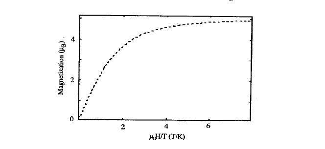
Figure 2.22. Paramagnetic magnetization curve \((B)_{5/2}(x)\) for ions of ferric iron (Fe3+, \(J = S = 5/2\)).
randomly orientated moments. At high temperatures \(B_{J}(x) \approx (J + 1)x/3J\), so that
\(\langle m\rangle = \frac{g^{2}\mu_{\text{B}}^{2}J(J + 1)}{3k_{\text{B}}T}\mu_{0}H\). (2.96a)
The corresponding Curie law susceptibility (1.21) is
\(\chi = \frac{\mu_{0}}{3} \frac{m_{\text{eff}}^{2}}{k_{\text{B}}T} \frac{N}{V}\) (2.96b)
where \(N/V\) is the number of ions per magnet volume. This establishes a paramagnetic ionic moment
\(m_{\text{eff}} = g\sqrt{J(J + 1)}\mu_{\text{B}}\) (2.97)
which is somewhat larger than the Zeeman moment \(m = Jg\mu_{\text{B}}\) (compare with (1.20)). In terms of the effective Bohr magneton number, \(m_{\text{eff}} = p_{\text{eff}}\mu_{\text{B}}\). Values of \(p_{\text{eff}}\) are included in tables 2.4 and 2.5. In laboratory fields at room temperature, the average moments predicted by (2.96a) are fairly small. For example, putting \(T = 300\ K\), \(J = 1/2\), \(g = 2\) and \(\mu_{0}H = 1\ T\) yields \(\langle m\rangle = 0.0023\ \mu_{\text{B}}\). This indicates that exchange fields in magnets such as elemental iron have to be of the order of \(1000\ T\) to reproduce the observed ferromagnetic moments.
Ionic Charge Distribution
The temperature dependence of the rare-earth anisotropy largely originates from intra-multiplet excitations. Physically, finite-temperature intra-multiplet excitations make the ionic charge clouds more spherical, which reduces the net interaction with the anisotropic crystal field. In the limit of very high temperatures or for \(H = 0\), all \(2J + 1\) Zeeman states are occupied with equal probability, so the charge clouds are spherical and the anisotropy vanishes13.
13 Here \(H\) is an effective field which includes both Zeeman and exchange interactions.
In the intermediate regime the multipole moments are calculated from the expression
\(\langle Q_{n}\rangle = \frac{1}{Z} \sum_{J_{z}=-J}^{J} Q_{n}(J_{z}) \exp[-g\mu_{0}\mu_{\text{B}}H J_{z}/k_{\text{B}}T]\) (2.98)
where
\(Q_{2} = \theta_{2}\langle r^{2}\rangle_{4f}(3J_{z}^{2} - J(J + 1))\) (2.99)
\(Q_{4} = \theta_{4}\langle r^{4}\rangle_{4f}(35J_{z}^{4} - 30J(J + 1)J_{z}^{2} + 25J_{z}^{2}\)
\( - 6J(J + 1) + 3J^{2}(J + 1)^{2})\) (2.100)
and
\(Q_{6} = \theta_{6}\langle r^{6}\rangle_{4f}(231J_{z}^{6} - 315J(J + 1)J_{z}^{4} + 735J_{z}^{4} + 105J^{2}J(J + 1)^{2}J_{z}^{2}\)
\( - 525J(J + 1)J_{z}^{2} + 294J_{z}^{2} - 5J^{3}(J + 1)^{3}\)
\( + 40J^{2}(J + 1)^{2} - 60J(J + 1))\). (2.101)
In section 3.1.5 we will use these equations to discuss the temperature dependence of the magnetic anisotropy.


