

6. Applications: The Role of Magnetism in Modern Technology
Introduction to Magnetic Applications: From Theory to Practice
The original magnet application was the compass, where a freely suspended magnetic needle responded to the torque exerted on it by the field of the Earth. The permanent magnets used in most modern applications, however, serve to generate a magnetic field rather than respond to one. Magnets are useful precisely because they can deliver flux into the region of space known as the air - gap with no continuous expenditure of energy. The magnetic flux density \(B_{0}\) in the air - gap, equal to \(\mu_{0}H_{0}\), is the natural field to consider here because flux is conserved in a magnetic circuit, and forces on electric charges and magnetic moments all depend on \(B\). One way to classify magnet applications is by the nature of the flux distribution in the air - gap; it may be static or time - dependent, uniform or non - uniform. We now consider each case in more detail.
A static uniform field may be used to generate torque or align pre - existing magnetic moments since \(\boldsymbol{\Gamma}=\boldsymbol{m}\times\boldsymbol{B}\). On an atomic scale it produces Zeeman splitting of atomic and nuclear energy levels, which is the quantum equivalent of aligning the spins. Charged particles moving through the uniform field with velocity \(\boldsymbol{v}\) are deflected by the Lorentz force \(\boldsymbol{F}=q\boldsymbol{v}\times\boldsymbol{B}\), which causes them to move in a helix. When the charged particles are electrons confined to a conductor of length \(L\), they may constitute a current \(I\) flowing perpendicular to the field and the Lorentz force then leads to the familiar expression \(F = BIL\). This is the basis of electromagnetic drives. Conversely, moving a conductor through the uniform field produces an induced electromotive force (emf) given by Faraday's law of electromagnetic induction \(\varepsilon=-\frac{d\Phi}{dt}\), where \(\Phi = BA\) is the flux threading the circuit of which the conductor forms a part.
Spatially non - uniform fields offer another series of useful effects. They exert a force on a magnetic moment given by the gradient force \(\boldsymbol{F}=-\nabla(\boldsymbol{m}\cdot\boldsymbol{B})\). They also exert non - uniform forces on moving charged particles, which can be used to focus ion or electron beams or generate electromagnetic radiation from beams passing through the inhomogeneous field. The ability of rare - earth permanent magnets to generate complex flux patterns
with rapid spatial fluctuations (\(\nabla B>100\ T\ m^{-1}\)) is unsurpassed by any electromagnet. This point can be appreciated by considering the Amperian surface current, \(800\ kA\ m^{-1}\), which is equivalent to a long magnet with \(\mu_{0}M\approx1\ T\). Solenoids, whether resistive or superconducting, need to be several centimetres in diameter and length to accommodate the requisite ampere - turns. It is impractical to use them to generate field gradients of \(1\ T\ m^{-1}\) or more. Yet permanent magnet structures can be assembled from blocks of rare - earth or ferrite magnets in direct contact with any desired orientation.
Time - varying fields are produced by displacing or rotating the magnets. A field which varies in time can be used to induce an emf according to Faraday's law or produce eddy currents in a static conductor and exert forces on those currents. If it is spatially non - uniform, it can exert a time - dependent force on a magnetic moment or particle beam. Applications include magnetic switches and measurements of physical properties as a function of field.
A representative selection of the enormous range of applications which exploit the various effects is given in table 6.1. Certain reputed benefits of magnetic fields, such as use of magnets in acupuncture, pain control, electrochemistry, suppression of wax formation in oil wells or control of limescale deposits in pipes carrying hard water are difficult to classify. Magnets still carry an aura of mystery from their archaic past. 'Animal magnetism' provides an etymological link with hypnotism. Many of the unexplained influences of magnets may be placebo effects, but for some there is more serious evidence. Although the underlying mechanisms have yet to be identified, they will probably turn out to be related to one or other of those mentioned above. These are good areas for scientific investigation. A closed mind learns nothing.
Static vs. Dynamic Magnetic Operation: Key Differences and Uses
Viewed from the standpoint of the permanent magnet, the various applications are classified as static or dynamic according to whether the working point in the second quadrant of the hysteresis loop is fixed or moving. The position of the working point t depends on the magnitude of the \(H'\) field to which the magnet is subjected, which depends in turn on the shape of the magnet, the form of the air - gap and the rest of the magnetic circuit and any externally applied field. The working point will change whenever magnets move relative to each other, when the air - gap changes or when there are time - varying currents.
A magnetic circuit for any application will comprise magnets, air - gap and possibly soft iron to guide the flux. Some key ideas can be introduced by considering the simple magnetic circuit of figure 4.23. The circuit directs flux produced by the permanent magnet of length \(l_{\text{m}}\) and cross - section \(A_{\text{m}}\) through the soft - magnetic material into the air - gap of length \(l_{\text{g}}\) and cross - section \(A_{\text{g}}\). If there is no flux leakage, \(\nabla\cdot\boldsymbol{B}\approx0\) gives \[B_{\text{m}}A_{\text{m}}=-B_{\text{g}}A_{\text{g}}\](6.1)
Table 6.1. Examples of permanent magnet applications.
| Field | Magnetic effect | Static/ dynamic | Application |
|---|---|---|---|
| Uniform | Zeeman splitting | Static | Magnetic resonance imaging |
| Torque | Static | Magnetic powder alignment | |
| Hall effect, magnetoresistance | Static | Sensors | |
| Force on conductor | Dynamic | Motors, actuators, loudspeakers | |
| Non - uniform | Induced emf | Dynamic | Generators, microphones |
| Forces on charged particles | Static | Beam control, radiation sources (microwave, UV, x - ray) | |
| Force on paramagnet | Dynamic | Mineral separation | |
| Force on magnet | Dynamic | Holding magnets | |
| Variable field | Dynamic | Bearings, couplings, maglev | |
| Time - varying | Force on iron | Dynamic | Switchable clamps |
| Eddy currents | Dynamic | Brakes, metal separation |
Furthermore, if the soft material is ideal insofar as it has infinite permeability and \(H_{\text{m}}\) is the value of \(H'\) in the magnet, Ampère's law \(\int\boldsymbol{H}\cdot d\boldsymbol{l}=0\) gives (section 2.1.7.2) \[H_{\text{m}}l_{\text{m}}=H_{\text{g}}l_{\text{g}}\] (6.2)
Multiplying the above two equations and using the fact that \(B_{\text{g}}=\mu_{0}H_{\text{g}}\), \[B_{\text{m}}H_{\text{m}}V_{\text{m}}=-B_{\text{g}}^{2}V_{\text{g}}/\mu_{0}\] (6.3) where \(V_{\text{m}}\) and \(V_{\text{g}}\) represent the volumes of the magnet and the gap. The flux in the air - gap is maximized and optimum use made of the magnetic material when the product \(B_{\text{m}}H_{\text{m}}\) is maximum; hence the emphasis on energy product as a figure of merit. Dividing (6.1) by (6.2), we obtain the equation for the load line \(B_{\text{m}}(H_{\text{m}})\) (figure 4.21) whose negative slope \[-B_{\text{m}}/H_{\text{m}}=\mu_{0}A_{\text{g}}l_{\text{m}}/A_{\text{m}}l_{\text{g}}\] (6.4) is known as the permeance coefficient. The working point where the \(B - H'\) loop of a particular material intersects the load line is therefore determined by the geometrical dimensions of the magnet and air - gap. As materials improved, the magnets grew shorter and fatter to work near their \((BH)_{\text{max}}\) point. The working point corresponding to \((BH)_{\text{max}}\) for an isolated magnet with an ideal square loop is at permeance \(\mu_{0}\). There \(B = B_{\text{r}}/2\) and \(H=-M_{\text{r}}/2\), so the demagnetizing factor \(D\) should be exactly \(1/2\). A cylindrical magnet with an effective demagnetizing factor has a height/diameter ratio of 0.47. A squat cylinder is the new magnet archetype, replacing the horseshoe (figure 1.4).
In practice, there are some flux losses in the circuit of figure 4.23, so a factor \(\beta\) is introduced on the left – hand side of (6.1). Furthermore, the soft material will not be ideal so another factor, \(\alpha\), is introduced on the left – hand side of (6.2). Typically, \(\alpha\) is in the range 0.7 – 0.95, but \(\beta\) may be anywhere from 0.2 to 0.8. Generally, it is advantageous to position the magnets as close as possible to the air – gap. Rare – earth permanent magnets are particularly suited for use in ironless magnetic circuits where the flux is essentially confined to the air – gap and to the magnets themselves. Leakage is minimized and the magnet is used as effectively as possible. By suitable circuit design, flux concentration can be achieved whereby the flux density in the working volume can exceed the remanence of the magnet.
The analogy between magnetic and electric circuits, introduced in section 4.3.1, can be exploited as an aid to calculation of static configurations. This rests on the similarity between Ampere’s law \(\oint\boldsymbol{H}\cdot d\boldsymbol{l}=0\) in the absence of conduction currents and the corresponding result for the electric field \(\oint\boldsymbol{E}\cdot d\boldsymbol{l}=0\) in the absence of changing magnetic fields. The corresponding continuity equations are \(\nabla\cdot\boldsymbol{B}=0\) and \(\nabla\cdot\boldsymbol{j}=0\), where \(\boldsymbol{j}\) is the electric current density. The magnetic potential difference, defined by \(\varphi_{ab}=\int_{a}^{b}\boldsymbol{H}\cdot d\boldsymbol{l}\), is measured in amperes. This is a useful concept provided no conduction currents are present. The permanent magnet itself is the source of magnetomotive force (mmf), the magnetic analogue of emf, as it is the only segment of the circuit where the magnetic potential rises, because \(\boldsymbol{H}\) is oppositely directed inside and outside the magnet (figure 1.2, section 4.3). The magnetic flux \(\Phi\) is the equivalent of current and the reluctance \(R(=\varphi/\Phi)\) is the equivalent of resistance. The reluctance of a short air – gap, for instance, is
\(R_{g}=\varphi_{g}/\Phi_{g}=l_{g}/\mu_{0}A_{g}\). (6.5)
The magnet has an internal reluctance determined by its working point on the \(B:H\) loop (figure 4.22); \(R_{m}=\varphi_{m}/\Phi_{m}\). The equivalent circuit of figure 4.23(b) illustrated the principle of matching the air – gap reluctance to the desired working point of the magnet. Figure 4.23(c) showed the equivalent circuit allowing for non – zero reluctance of the soft segments and flux losses. These losses are much more severe in magnetic circuits than in their electrical counterparts because the relative permeability of iron \(\mu_{r}\approx10^{3}-10^{4}\) is much less than the conductivity of copper relative to that of air. We have many good electrical insulators, but the only magnetic insulators are type I superconductors (\(\mu_{r}=0\)). Furthermore, the high permeabilities of soft magnets do not lead to magnetizations exceeding \(M_{s}\).
On account of their square loops, oriented ferrite and rare – earth magnets are particularly well suited for dynamic applications that involve changing flux density in the permanent magnet. Ferrites and bonded metallic magnets also minimize eddy current losses. For mechanical recoil (figure 6.1), the air – gap changes during operation from a narrow one with reluctance \(R_{1}\) to a wider one with reluctance \(R_{2}\). After several cycles, the working point follows a stable
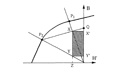
Figure 6.1. The hysteresis loop showing the working point for a dynamic application with mechanical recoil.
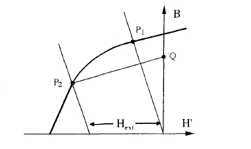
Figure 6.2. Hysteresis loop showing the working point for a dynamic application with active recoil.
and almost linear trajectory, represented by the line \(P_{2}Q\) whose slope is known as the recoil permeability \(\mu_{\text{R}}\). The recoil permeability is \(2 - 6\mu_{0}\) for alnicos, but it is barely greater than \(\mu_{0}\) for oriented ferrite and rare - earth magnets. \(XY\) represents the useful flux change in the gap and \(YZ\) the leakage flux that is wasted. The area \(XX'Y'Y\) is a measure of the recoil product \((BH')_{u}\), which is twice the useful recoil energy in the gap and is maximized when \(X\) bisects \(P_{2}Q\). \((BH')_{u}\) will always be less than \((BH)_{\text{max}}\), but it approaches that limit in materials with high coercivity and a square loop where the recoil permeability approaches \(\mu_{0}\).
Active recoil occurs in permanent magnet motors and other devices where the magnets are subject to an \(H\) field during operation as a result of currents in the copper windings. The field is greatest at start - up or in the stalled condition. Active recoil is represented by a displacement of the reluctance line along the \(H\) - axis (figure 6.2). Provided \(\mu_{0}H_{\text{c}}\) exceeds \(B_{\text{r}}\), it is possible to
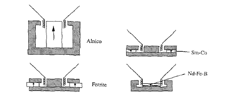
Figure 6.3 . The influence of permanent-magnet properties on the design of loudspeakers.
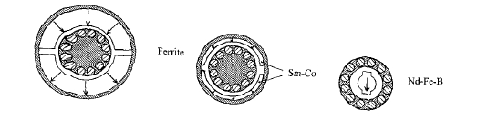
Figure 6.4 . The influence of permanent-magnet properties on the design of dc motors
drive the working point momentarily into the third quadrant of the \(B - H\) loop without de - magnetizing the permanent magnet. The intrinsic coercivity may be as important a figure of merit as \((BH')_{\text{max}}\) in this type of application.
Electrical machines are generally modelled using the vector potential \(\boldsymbol{A}\), using the finite - difference and finite - element methods presented in section 4.3.
Magnetic Materials in Applications: Selection, Performance, and Innovations
Figures 6.3 and 6.4 vividly illustrate the influence of permanent magnet material on device design. Not only can the device be made smaller with high - energy - product magnets, but the number of parts can be reduced. For example, the magnets of a brushless dc motor can be moved to the rotor and the magnets moulded together with the shaft and gear in one piece. There is a trend towards miniaturization coupled with moving - magnet designs. These have the virtues that moving magnets have low inertia and the stationary windings can be thermally heat - sunk. The advantage of the magnet may be appreciated by comparing a small disc - shaped magnet with a coil having the same moment. A disc with diameter 8 mm and height 2 mm made of a material with \(M = 1\ MA\ m^{-1}\) has \(m\approx0.1\ A\ m^{2}\). The equivalent current loop, \(m = IA\), would require 2000 ampere - turns, an impossible proposition in these dimensions.
Table 6.2. Mechanical, electrical and thermal properties of permanent magnets. \(E =\) Young's modulus, \(\rho_{e}=\) resistivity.
| \(\rho\) (kg m-3) | \(\alpha\) (10-6 C-1) | \(\rho_{e}\) (\(\mu\Omega\) m) | \(M_{\text{s}}^{-1}\text{d}M_{\text{s}}/\text{d}T\) (% C-1) | \(H_{\text{c}}^{-1}\text{d}H_{\text{c}}/\text{d}T\) (% C-1) | \(T_{\text{max}}\) (°C) | |
|---|---|---|---|---|---|---|
| SrFe12O19 sintered | 4300 | 10 | 108 | -0.20 | 0.45 | 280 |
| SrFe12O19 bonded | 3600 | — | — | -0.20 | 0.45 | 150 |
| Alnico 5 cast | 7200 | 12 | 0.5 | -0.02 | 0.03 | 500 |
| SmCo5 sintered | 8400 | 11 | 0.6 | -0.04 | -0.02 | 260 |
| Sm2Co17 sintered | 8400 | 10 | 0.9 | -0.03 | -0.20 | 350 |
| Nd2Fe14B sintered | 7400 | -2 | 1.5 | -0.13 | -0.60 | 150 |
| Nd2Fe14B bonded | 6000 | — | 200 | -0.13 | -0.60 | 120 |
a Intergrown with the 1:5 phase.
The most important commercial applications of permanent magnets are in motors, actuators and other electromagnetic machines. A vast range of motors can be designed with magnets, their power ranging from microwatts, for wristwatch motors, to hundreds of kilowatts, for industrial drives. The high energy product and high anisotropy of the rare - earth permanent magnets makes it possible to realize compact, low - inertia, high - torque devices—stepper motors, actuators, brushless dc motors—which are the means for electronically regulated motion control. Global production of rare - earth magnets is about \(15\times10^{3}\) tonnes/year. Ferrites are produced in huge quantities for low - cost motors for consumer products, including automobiles. Ferrite production has been doubling every 3 - 5 years, and is currently about \(5\times10^{5}\) tonnes/year.
The magnets in electrical machines can be subject to temperatures in excess of 100 °C. Magnetization and coercivity naturally decline as the Curie point is approached. The temperature coefficients of these quantities around the ambient temperature are listed in table 6.2 for magnets made of different materials. Not all the loss is necessarily recoverable on returning to the ambient temperature; there can be irreversible losses associated with thermal cycling. The maximum temperatures at which the materials can be safely used are also indicated in table 6.2. The limit for Nd2Fe14B is lower than for any of the others because of its relatively low Curie point and high temperature coefficients. These are difficulties to be overcome by astute engineering design.
Unlike the old steel magnets and alnicos, ferrites and rare - earth magnets with wide, square hysteresis loops have the property that the field of one magnet does not significantly perturb the magnetization of a neighbouring magnet. This is because the longitudinal susceptibility is zero for a square hysteresis loop and the transverse susceptibility \(M_{\text{s}}/H_{0}\) is only of the order of 0.1, since the anisotropy field \(H_{0}=2K_{1}/\mu_{0}M_{\text{s}}\) (3.7) is much greater than the magnetization (table 5.18). Hence, for example, the directions of magnetization of two blocks of \(\text{SmCo}_{5}\) in contact, with their easy directions perpendicular, will deviate less than a degree from the easy axes. For \(\text{Nd}_{2}\text{Fe}_{14}\text{B}\) or \(\text{SrFe}_{12}\text{O}_{19}\), the deviation is a few degrees. A consequence of the rigidity of the magnetization is that the superposition of the induction of rare - earth permanent magnets is linear and the magnetic material is effectively transparent, behaving like a vacuum with permeability \(\mu_{0}\). Transparency and rigidity of the magnetization greatly simplify the design of magnetic circuits. Throughout this chapter, permanent magnets are represented by unshaded blocks with an arrow to show the direction of magnetization.
We now look at some specific applications in more detail.


