
2.4 Itinerant Magnetism: Basics and Concepts
The magnetic moment of metallic permanent magnets originates largely or exclusively from transition-metal 3d electrons. As metallic 3d electrons are delocalized or itinerant, they cannot be described in terms of the localized Heisenberg model. The delocalized Hartree–Fock approximation (section 2.1.6.1) is a better starting point. As in 3d oxides, the orbital moment of itinerant 3d electrons is effectively quenched. Typical values are of order \(0.1\ \mu_{\text{B}}\), so that the Landé \(g\) factor is close to 2. This means that the moment of 3d atom, measured in \(\mu_{\text{B}}\), is nearly equal to the number of unpaired electrons.
As mentioned in section 1.2.1.2, itinerant moments are difficult to predict. This is in contrast to the moments of ferromagnetic oxides, which are given by the atomic structure and composition. The example of \(ZrZn_{2}\) consists of two non-magnetic elements, but is weakly ferromagnetic below \(T_{\text{C}} = 17\ \text{K}\), whereas the isostructural compound \(YNi_{2}\) is paramagnetic at all temperatures. Another example is iron: bcc iron has a magnetic moment of \(2.22\ \mu_{\text{B}}\) per atom, whereas bulk fcc iron is probably antiferromagnetic. In practice, the number of itinerant \(\uparrow\) and \(\downarrow\) electrons is determined from independent-electron band-structure calculations.
The problem is that itinerant 3d electrons are temporarily captured in virtual bound states around the transition-metal cores. This causes the 3d electrons to suffer a time delay in their general translational motion and gives them some localized character. This complicates the distinction between intra-atomic and (effective) inter-atomic exchange. On the other hand, moment formation is supported by energies of order \(1\ \text{eV}\), whereas Heisenberg exchange energies are of at most order \(0.1\ \text{eV}\). As a consequence, ferromagnetic moments are fairly well conserved at the Curie temperature. An exception are very weak itinerant ferromagnets, where the thermal destruction of the spontaneous magnetization is accompanied by a nearly complete reduction of the magnetic moment.
Table 2.14 summarizes the two limits of localized and itinerant magnetism. The formation of itinerant moments is not restricted to iron-series 3d electrons, but itinerant 4d, 5d and 5f moments are comparatively small. Note that itinerant moments do not necessarily yield ferromagnetism. For instance, chromium and manganese are itinerant antiferromagnets having complicated spin structures below the respective Néel temperatures, 312 K and 95 K.
This section is divided into three parts. In section 2.4.1 we investigate the free-electron limit, which provides a qualitative understanding of itinerant magnetism but is unable to yield quantitative predictions. In section 2.4.2 we focus on the moment of real metals and section 2.4.3 is devoted to the Curie temperature of itinerant magnets.
Free Electron Magnetism Explained
The simplest approach in order to understand the metallic band structure is the 1929 free-electron theory of Bloch. It describes the limit of very high electron densities, where the kinetic energy dominates all electrostatic energy contributions. Since free electrons are completely delocalized, this model is a good starting point for the discussion of itinerant magnetism. Although high-density free electron gases are Pauli paramagnets, the Hartree–Fock approximation yields electrostatic corrections which reveal the origin of itinerant ferromagnetism.
Density of States (DOS)
The high electrical conductivity of metals indicates the presence of delocalized, itinerant electrons. In other words, the attractive potential of the positively charged nuclei is insufficient to hold the outer electrons in atomic orbitals. The simplest and most extreme approximation is to neglect the influence of the electrostatic potential altogether and treat the conduction electrons as a free-electron gas. Putting \(V(\mathbf{r}) = 0\) in (2.14) we obtain the plane-wave solutions
\(\psi_{\mathbf{k}}(\mathbf{r}) = \frac{1}{\sqrt{\Omega}} e^{i\mathbf{k} \cdot \mathbf{r}}\) (2.152)
where \(\Omega = L_{0}^{3}\) is the volume of the solid.
The energy of an electron with wavevector \(\mathbf{k}\) is \(E_{\mathbf{k}} = \hbar^{2}k^{2}/(2m_{\text{e}})\), but the number of wavevectors is restricted by the boundary condition \(\psi_{\mathbf{k}}(\mathbf{r} + L_{0}\mathbf{e}_{x}) = \psi_{\mathbf{k}}(\mathbf{r} + L_{0}\mathbf{e}_{y}) = \psi_{\mathbf{k}}(\mathbf{r} + L_{0}\mathbf{e}_{z}) = \psi_{\mathbf{k}}(\mathbf{r})\). This requirement is satisfied by using periodic boundary conditions \(k_{x}L_{0} = 2\pi n_{x}\), \(k_{y}L_{0} = 2\pi n_{y}\), and \(k_{z}L_{0} = 2\pi n_{z}\), so that \(k\) space turns out to be divided into cells of volume \(\Delta k = (2\pi / L_{0})^{3}\). The electrons obey Fermi–Dirac statistics, which permit each orbital to be occupied by at most one \(\uparrow\) electron and one \(\downarrow\) electron. This means that \(k\) states are filled

Figure 2.36. Free-electron density of states for ↑ and ↓ electrons.
as milk is poured into a bowl, until the Fermi energy \(E_{\text{F}} = \hbar^{2}k_{\text{F}}^{2}/2m_{\text{e}}\) is reached. The Fermi level is determined by the density \(N/L_{0}^{3}\) of electrons occupying the \(k\)-space cells, so that the \(k\)-space volume \(4\pi k_{\text{F}}^{3}/3\) of the Fermi sphere yields \(k_{\text{F}} = (3\pi^{2}N/\Omega)^{1/3}\). Typical Fermi energies are \(E_{\text{F}} = 3.24\ \text{eV}\) (\(37700\ \text{K}\)) for \( \text{Na}\) and \(E_{\text{F}} = 7.00\ \text{eV}\) (\(81600\ \text{K}\)) for \( \text{Cu}\).
A way of visualizing band-structure results is to consider the density of states \( \mathcal{D}(E)\), that is the number of \(k\) states per energy interval. For free electrons it has the parabolic form (figure 2.36)
\(\mathcal{D}(E) = \frac{3}{2} \frac{N}{\Omega} \sqrt{\frac{E}{E_{\text{F}}}}\) (2.153)
where \( \mathcal{D}(E_{\text{F}}) = 3N/(2\Omega E_{\text{F}})\). In the paramagnetic state, the number of \(\uparrow\) electrons equals that of \(\downarrow\) electrons and the net moment is zero, but external magnetic fields \( \mathbf{H} = H\mathbf{e}_{z}\) transfer \(\downarrow\) electrons to \(\uparrow\) states and produce a small magnetization (Zeeman interaction). In the density of states, this is seen as a relative shift of the \(\uparrow\) and \(\downarrow\) subband densities of states (figure 2.36).
Conduction electrons of simple metals such as \( \text{Na}\), \( \text{Cu}\) and \( \text{Au}\) are free-electron-like, since the \(s\) bands are broad and the kinetic energy dominates the electrostatic interaction. From the scaling behaviour of the kinetic and electrostatic energies, \(k_{\text{F}}^{2} \propto (N/\Omega)^{2/3}\) and \(1/r \propto (N/\Omega)^{1/3}\), respectively, where \(r\) is an average interelectronic distance, we see that the free-electron theory is a high-density approach. By comparison, itinerant electrons originating from the partly filled inner shells of transition-metal elements feel rather strong ionic potentials \(V(r)\), which gives rise to major deviations from the free-electron predictions.
Pauli Paramagnetism
The spin polarization indicated by figure 2.36 reflects the competition between the Zeeman energy and the kinetic energy. The Pauli susceptibility \(\chi_{\text{P}} = \partial M/\partial H\), which describes the outcome of this competition, is of great
importance, because it makes it possible to estimate the exchange field \(M_{s}/\chi_{\text{P}}\) necessary to create ferromagnetism. Elementary free-electron theory yields
\(E = \frac{m_{\text{e}}\alpha^{2}c^{2}}{5} \sum_{\sigma} k_{\sigma}^{2} a_{0}^{2} N_{\sigma} - \mu_{0}\mu_{\text{B}}H(N_{\uparrow} - N_{\downarrow})\) (2.154)
where the sum includes the two spin directions and the parameters \(k_{\uparrow}\) and \(k_{\downarrow}\) are the spin-up and spin-down Fermi wavevectors defined by \(E_{\sigma} = \hbar^{2}k_{\sigma}^{2}/2m_{\text{e}}\). It is convenient to rewrite the energy (2.154) in terms of the total number of electrons, \(N = N_{\uparrow} + N_{\downarrow}\), and the spin polarization \(s = (N_{\uparrow} - N_{\downarrow})/(N_{\uparrow} + N_{\downarrow})\). The magnetization is then given by \(M = Ns\mu_{\text{B}}\). Linearization of (2.154) with respect to \(s\) and taking into account the fact that \(k_{\sigma}^{2} = 6\pi^{2}N_{\sigma}/\Omega\) yields
\(\frac{E}{N} = \frac{m_{\text{e}}}{2} \alpha^{2}c^{2} \frac{k_{\text{F}}^{2}a_{0}^{2}}{3}s^{2} - \mu_{0}\mu_{\text{B}}Hs\) (2.155)
where a physically unimportant zero-point energy has been omitted. Putting \(H = 0\) in this equation yields an energy minimum at \(s = 0\), that is a paramagnetic ground state. For \(H \neq 0\), the minimization of (2.155) yields the spin polarization \(N\mu_{\text{B}}s = \chi_{\text{P}}H\) where
\(\chi_{\text{P}} = \frac{\alpha^{2}}{\pi} k_{\text{F}}a_{0}\). (2.156)
The product \(k_{\text{F}}a_{0}\) is of order one, but the involvement of Sommerfeld's constant \(\alpha = 1/137\) causes the free-electron Pauli susceptibility to be very small.
Exchange-enhanced Pauli Paramagnetism
In section 2.1.5 we have seen that ferromagnetism is caused by many-body interactions of type (2.49). In lowest-order perturbation theory, the mutual Coulomb repulsion of the electrons is included by using Slater determinants constructed from the interaction-free one-electron wavefunctions. For free electrons, one obtains
\(E = \frac{m_{\text{e}}\alpha^{2}c^{2}}{2} \sum_{\sigma} \left(\frac{3k_{\sigma}^{2}a_{0}^{2}}{5} - \frac{3k_{\sigma}a_{0}}{\pi}\right) N_{\sigma} - \mu_{0}\mu_{\text{B}}H(N_{\uparrow} - N_{\downarrow})\). (2.157)
This equation differs from (2.154) by the interaction term \(-3k_{\sigma}a_{0}/\pi\). Expressing the total energy (2.157) in terms of \(N\) and \(s\) yields, for \(H = 0\), the curves in figure 2.37, which predict ferromagnetism for small \(k_{\text{F}}\), that is for low electron densities.
To determine the onset of ferromagnetism we expand \(E'\) into powers of \(s\)
\(\frac{E}{N} = \frac{m_{\text{e}}}{2} \alpha^{2}c^{2} \frac{k_{\text{F}}^{2}a_{0}^{2}}{3} \left(1 - \frac{1}{\pi k_{\text{F}}a_{0}}\right) s^{2} - \mu_{0}\mu_{\text{B}}Hs\). (2.158)
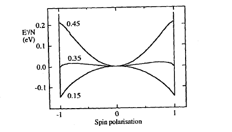
Figure 2.37. Magnetic energy per free electron for different values of \(k_{\text{F}}a_{0}\).
Putting \(H = 0\) in this equation we see that the paramagnetic \(s = 0\) energy minimum vanishes at \(\pi k_{\text{F}}a_{0} = 1\). This means that the Hartree–Fock free-electron gas is ferromagnetic when
\(\frac{1}{\pi k_{\text{F}}a_{0}} > 1\). (2.159)
An alternative derivation of this criterion is based on the comparison of equations (2.155) and (2.158), which yields the enhanced Pauli susceptibility
\(\chi = \frac{\chi_{\text{P}}}{1 - 1/\pi k_{\text{F}}a_{0}}\) (2.160)
for \(\pi k_{\text{F}}a_{0} > 1\) and ferromagnetism for \(\pi k_{\text{F}}a_{0} < 1\).
Equation (2.159) predicts ferromagnetism for simple bcc and fcc metals with atomic radii larger than 281 pm (2.81 Å) and 289 pm (2.89 Å), respectively. In fact, heavy alkali metals such as rubidium and caesium, which come closest to this threshold, are paramagnetic, whereas the atomic radii of the ferromagnetic 3d elements Fe, Co and Ni are about 125 pm (1.25 Å). This means that the description of itinerant 3d magnetism in terms of interacting free electrons is inadequate, although the key feature of the approach, namely the susceptibility enhancement due to the electrostatic interaction, carries over to real 3d metals.
Band Structure and Magnetic Moments
A more accurate description of itinerant magnetism requires the use of more reasonable one-electron wavefunctions than plane waves. The simplest approach is the Stoner theory, which predicts ferromagnetism when the paramagnetic density of states (DOS) exceeds some critical value \( \mathcal{D}_{\text{p}}(E_{\text{F}}) > 1/l\), where \(l \approx 1\ \text{eV}\). Indeed, we will see that the late 3d elements have their paramagnetic Fermi levels at a pronounced d-band peak where this Stoner criterion is satisfied.
Tight-binding 3d Bands
By analogy to (2.47), delocalized wavefunctions can be constructed from localized Wannier functions:
\(\Psi_{\mathbf{k}\mu}(\mathbf{r}) = \frac{1}{\sqrt{N}} \sum_{i} \exp(i\mathbf{k} \cdot \mathbf{R}_{i})\varphi_{\mu}(\mathbf{r} - \mathbf{R}_{i})\) (2.161)
where the index \(\mu\) indicates from which atomic orbital the band derives26. The Wannier orbitals \(\varphi_{\mu}(\mathbf{r})\) differ from the atomic wavefunctions by long-range oscillations. The magnitude of the oscillations increases with the overlap of the atomic wavefunctions and is particularly large for valence-band s electrons. On the other hand, the overlap of atomic 3d wavefunctions in metals is comparatively small, which makes it possible to interpret the Wannier orbitals as atomic wavefunctions. This approach is known as the LCAO (linear combination of atomic orbitals) or tight-binding approximation.
The overlap of the atomic wavefunctions leads to the broadening of the atomic 3d levels into bands. The tight-binding band structure is given by the energy matrix \(\langle\Psi_{\mathbf{k}\mu}|H|\Psi_{\mathbf{k}\mu'}\rangle = \delta_{\mathbf{k}\mathbf{k}'}E_{\mu\mu'}(\mathbf{k})\) where
\(E_{\mu\mu'}(\mathbf{k}) = \sum_{i} \exp(i\mathbf{k} \cdot \mathbf{R}_{i}) \int \varphi_{\mu}^{*}(\mathbf{r})H\varphi_{\mu'}(\mathbf{r} - \mathbf{R}_{i}) d\mathbf{r}\). (2.162)
It is convenient to divide the one-electron Hamiltonian \(H = H_{0} + \Delta H\) into an atomic part \(H_{0}\) and a perturbative part \(\Delta H\) containing all remaining energy contributions. Restricting ourselves to nearest-neighbour interactions we obtain
\(E_{\mu\mu'} = E_{0}\delta_{\mu\mu'} + V_{\mu\mu'} + \sum_{i} \exp(i\mathbf{k} \cdot \mathbf{R}_{i})T_{\mu\mu'}(\mathbf{R}_{i})\) (2.163)
where \(E_{0}\) is the energy of the atomic d levels and the summation is restricted to nearest neighbours. The behaviour of 3d metals is largely determined by hopping integrals
\(T_{\mu\mu'}(\mathbf{R}_{i}) = \int \varphi_{\mu}^{*}(\mathbf{r} - \mathbf{R}_{i})\Delta H(\mathbf{r})\varphi_{\mu'}(\mathbf{r}) d\mathbf{r}\). (2.164)
By comparison, the crystal-field or shift integrals
\(V_{\mu\mu'} = \int \varphi_{\mu}^{*}(\mathbf{r})\Delta H(\mathbf{r})\varphi_{\mu'}(\mathbf{R}) d\mathbf{r}\) (2.165)
are of secondary importance (Mott 1974).
26 Note that (2.161) is an alternative to writing Bloch wavefunctions \(\Psi_{\mathbf{n}\mathbf{k}}(\mathbf{r}) = u_{\mathbf{n}\mathbf{k}}(\mathbf{r})\exp(i\mathbf{k} \cdot \mathbf{r})\).
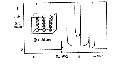
Figure 238. Total density of states for chains of 3d atoms.
The DOS \( \mathcal{D}(E)\) we are seeking is obtained by diagonalizing the matrix \(E_{\mu\mu'}(\mathbf{k})\) for each \(\mathbf{k}\) point and counting the number of eigenstates having energies between \(E\) and \(E + dE\). A simple example is a hypothetical chain compound where the 3d atoms form well separated parallel chains. Neglecting the crystal-field integrals we obtain from (2.163)
\(E_{\mu\mu'} = E_{0}\delta_{\mu\mu'} + \cos(k_{z}a)\begin{pmatrix}V_{\text{dd}\sigma} & 0 & 0 & 0 & 0 \\ 0 & V_{\text{dd}\pi} & 0 & 0 & 0 \\ 0 & 0 & V_{\text{dd}\pi} & 0 & 0 \\ 0 & 0 & 0 & V_{\text{dd}\delta} & 0 \\ 0 & 0 & 0 & 0 & V_{\text{dd}\delta}\end{pmatrix}\) (2.166)
where \(V_{\text{dd}\sigma}\), \(V_{\text{dd}\pi}\) and \(V_{\text{dd}\delta}\) are fundamental hopping integrals (Slater and Koster 1954). Since this matrix is diagonal for all \(\mathbf{k}\) vectors, it is easy to calculate the DOS from (2.166). Figure 2.38 reveals singularities in the DOS which are due to the one-dimensional character of the chains.
Since the matrix elements \(T_{\mu\mu'}(\mathbf{R})\) and the Slater–Koster integrals decrease with the inter-atomic distance, well separated 3d shells give rise to narrow bands and high densities of states. On the other hand, in section 2.1.6 we have shown that small one-electron energy differences, that is narrow bands, favour ferromagnetism. For this reason it is possible to estimate itinerant moments from the non-magnetic (paramagnetic) DOS.
Often it is desirable to predict the DOS directly from the atomic environment, without calculating the complete set of wavevector-dependent energy levels. A systematic real-space approach which solves this problem is based on the moments theorem by Cyrot-Lackmann of (1968). The theorem considers the \(m\)th moments \(\mu_{m} = \int E^{m} \mathcal{D}(E) dE\) of the DOS rather than the function \( \mathcal{D}(E)\). For example, the moments \(\mu_{0}\), \(\mu_{1}\) and \(\mu_{2}\) determine the maximum number of electrons in the band, the centre of gravity of the band and the bandwidth, respectively.
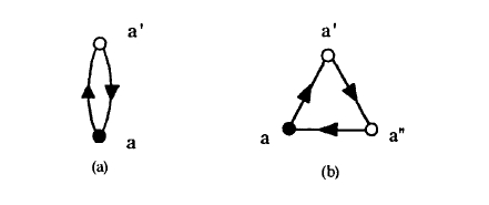
Figure 2.39. Elementary hopping loops: (a) a two-hop loop and (b) a three-hop loop.
The moments \(\mu_{m} = \sum_{a} \mu_{m}(a)\) are obtained from the local (site-projected) moments
\(\mu_{m}(a) = \langle\varphi_{a}|H^{m}|\varphi_{a}\rangle\) (2.167)
where \(a\) is a multi-index denoting site, spin and magnetic quantum number of the localized orbital \(|\varphi_{a}\rangle\)27. Utilizing the completeness of the localized orbitals and assuming a common d-electron centre of gravity \(\mu_{1} = 0\) we obtain
\(\mu_{m}(a) = \sum_{a',a''...} T(a,a')...T(a'',a)\). (2.168)
Here \(T(a_{1},a_{2})\) is the hopping integral connecting the orbitals \(a_{1}\) and \(a_{2}\), and the summation includes all closed loops having a length of \(m\) hops. The real-space expressions of the expressions
\(\mu_{2}(a) = \sum_{a'} T(a,a')T(a',a)\) (2.169a)
and
\(\mu_{3}(a) = \sum_{a',a''} T(a,a')T(a',a'')T(a'',a)\) (2.169b)
is shown in figure 2.39. Note that moments obtained from (2.168) are exact, even if \(m\) is much smaller than the total number of atoms in the solid. However, to reconstruct the density of states one needs a large number of moments if the peak structure is to be resolved properly.
In the case of d electrons, the \(m\)th moments contain factors
\(\left(\frac{1}{5}(V_{\text{dd}\sigma}^{2} + 2V_{\text{dd}\pi}^{2} + 2V_{\text{dd}\delta}^{2})\right)^{1/m}\) (2.170)
27 To calculate the expression \(\mu_{m} = \int E^{m} \mathcal{D}(E) dE\) we start from \(\mathcal{D}(E) = \int \delta(E - E_{k}) dk\), where \(k\) labels the electronic eigenstates of the solid. The \(\delta\)-function means that \(\mu_{m} = \int E_{k}^{m} dk\), but since the values \(E_{k}^{m} = \langle\psi_{k}|H^{m}|\psi_{k}\rangle\) are unknown we have to use the expansion \(|\psi_{k}\rangle = \sum_{a} c_{k,a}|\varphi_{a}\rangle\). This yields \(\mu_{m} = \sum_{a,a'} c_{k,a}^{*}c_{k,a'}\langle\varphi_{a}|H^{m}|\varphi_{a'}\rangle\) with the completeness relation \(\int c_{k,a}^{*}c_{k,a'} dk = \delta_{a,a'}\), the moments we are seeking. Since the derivation of the moments theorem does not involve Bloch wavefunctions, it applies equally well to periodic lattices, amorphous solids, clusters and surfaces.
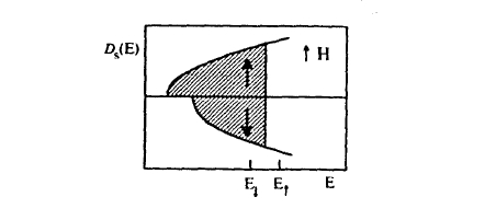
Figure 2.40. Asymmetry of the density of states: (a) \(\mu_{3} = 0\) and (b) \(\mu_{3} < 0\). As a guide for the eye, the arrows show some approximate Fermi levels.
which can be interpreted as effective \(m\)th order hopping integrals for \(\uparrow\) or \(\downarrow\) electrons. Restricting ourselves to nearest neighbours we have to consider \(z\) two-hop loops of the type in figure 2.39(a), so that \(\mu_{2} = zT_{(2)}^{2}\). Since the bandwidth \(W\) of rectangular bands obeys \(W^{2} = 12\mu_{2}\), we obtain the approximate relation
\(W = \sqrt{12z}T_{(2)}\). (2.171)
Numerically, this result is not very different from the relation \(W = 2zT_{(2)}\) valid for s bands in d-dimensional hypercubic lattices (\(z = 2d\)).
The third moment describes the asymmetry of the DOS (figure 2.40). Since hopping integrals are negative, the triangular real-space environment figure 2.39(b) yields a shift of the maximum of the DOS towards higher energies, as in figure 2.40(b). In the bcc structure there are no three-hop loops of the type in figure 2.39(b)28, so that the DOS is comparatively symmetric. By contrast, in the fcc structure there are 24 three-hop loops per site, and the skewing of the DOS is pronounced (see figure 2.46). We will see that this difference affects the magnetic behaviour of 3d metals.
Stoner Theory
To explain itinerant ferromagnetism we have to generalize the two-electron Coulomb repulsion in (2.43) to an electron gas of density \(n\):
\(V_{2}(\mathbf{r},\mathbf{r}') = \frac{e^{2}}{4\pi\epsilon_{0}} \int \frac{n(\mathbf{r})n(\mathbf{r}')}{|\mathbf{r} - \mathbf{r}'|} d\mathbf{r} d\mathbf{r}'\). (2.172)
Since the Pauli principle forbids the presence of two \(\uparrow\) electrons in a localized orbital, this equation gives rise to on-site interaction energies of the type \(U\hat{n}_{\uparrow}\hat{n}_{\downarrow}\). Here the \(\hat{n}_{\sigma}\) are the \(\uparrow\) and \(\downarrow\) particle-number operators acting on the many-body wavefunction and, as in section 2.1.5, \(U\) is the energy necessary to put a second electron of opposite spin on a localized orbital. In terms of the operator
28 Hopping integrals decrease rapidly with increasing inter-atomic distance. However, the bcc next-nearest neighbour distance is only 15% larger than that between nearest neighbours, so that next-nearest neighbour hopping is not necessarily negligible.
\(\hat{n} = \hat{n}_{\uparrow} + \hat{n}_{\downarrow}\), this Hubbard energy is equal to \(U\hat{n}^{2}/4 - U(\hat{n}_{\uparrow} - \hat{n}_{\downarrow})^{2}/4\), so that the on-site Coulomb repulsion favours moment formation.
Although the consideration of on-site repulsions yields a qualitative explanation of ferromagnetism, it does not circumvent the many-body character of the problem. In section 2.1.6.1 we saw that Hartree–Fock–Slater determinants establish a reasonable approximation in the metallic limit of strong inter-atomic hopping. Essentially, the determinants satisfy the Pauli principle but are constructed from one-electron wavefunctions. To transform the Coulomb interaction into an independent-electron potential we use the quantum-mechanical mean-field relation
\(\hat{n}_{\uparrow}\hat{n}_{\downarrow} = \hat{n}_{\uparrow}(\hat{n}_{\uparrow} + \hat{n}_{\downarrow}) + C\) (2.173)
where \(C\) is a negligible correlation term (cf 2.114). This means that the electrons move in some averaged interaction potential, but due to the involvement of \(\hat{n}_{\uparrow}\) and \(\hat{n}_{\downarrow}\) the one-electron potential is spin dependent.
The spin-dependent Coulomb potential favours ferromagnetism, but it has to compete against hopping-type one-electron energies incorporated into the paramagnetic DOS. Let us make the fair assumption that the paramagnetic DOS does not depend on the number of electrons in the two subbands. As in the free-electron case (figure 2.36), a magnetic field applied in the \(+e_{z}\) direction transfers electrons from the \(\downarrow\) to the \(\uparrow\) band. The energy of the electrons in the band is
\(E_{\text{B}} = \int_{0}^{E_{\uparrow}} E\mathcal{D}_{\uparrow}(E) dE + \int_{0}^{E_{\downarrow}} E\mathcal{D}_{\downarrow}(E) dE\) (2.174)
where \(E_{\uparrow}\) and \(E_{\downarrow}\) are the Fermi levels of the \(\uparrow\) and \(\downarrow\) subbands. \(\mathcal{D}_{\sigma}\) is the DOS per spin and atom; in terms of the crystal volume \(\Omega_{\text{T}}\) per transition-metal atom it is given by \(\mathcal{D}_{\sigma} = \Omega_{\text{T}}\mathcal{D}/2\). The total number of electrons and the spin polarization are given by \(E_{\uparrow}\) and \(E_{\downarrow}\):
\(\int_{0}^{E_{\uparrow}} \mathcal{D}_{\uparrow}(E) dE + \int_{0}^{E_{\downarrow}} \mathcal{D}_{\downarrow}(E) dE = N\) (2.175a)
\(\int_{0}^{E_{\uparrow}} \mathcal{D}_{\uparrow}(E) dE - \int_{0}^{E_{\downarrow}} \mathcal{D}_{\downarrow}(E) dE = sN\). (2.175b)
In the limit of small spin polarization we can replace the function \(\mathcal{D}_{\sigma}(E)\) by \(\mathcal{D}_{\sigma}(E_{\text{F}})\). Adding the Zeeman energy \(E_{Z}\) and neglecting a physically uninteresting zero-point energy, we obtain after a short calculation
\(E_{\text{B}} = \frac{N^{2}}{4\mathcal{D}_{\sigma}(E_{\text{F}})}s^{2} - \mu_{0}\mu_{\text{B}}N H s\). (2.176)
The number of electrons transferred from the \(\downarrow\) band to the \(\uparrow\) band is given by the Pauli susceptibility for a general density of states (cf (2.156))
\(\chi_{\text{P}} = \frac{2\mu_{0}\mu_{\text{B}}^{2}\mathcal{D}_{\sigma}(E_{\text{F}})}{\Omega_{\text{T}}}\). (2.177)
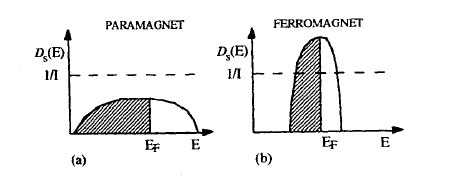
Figure 2.41. Schematic densities of states: (a) broad band and (b) narrow band. The Stoner criterion is satisfied when \( \mathcal{D}_{\sigma}(E)\) is larger than \(1/I\).
Equations (2.176) and (2.177) mean that the spin polarization created by a magnetic or exchange field \(H\) is proportional to \(\mathcal{D}_{\sigma}(E_{\text{F}})\).
According to Stoner (1938), the exchange interaction can be parametrized by the energy contribution
\(E_{\text{ex}} = -\frac{I}{4}(N_{\uparrow} - N_{\downarrow})^{2}\) (2.178)
where \(I \approx 1\ \text{eV}\) is the Stoner parameter. The structure of this term derives from the Coulomb repulsion (2.172), although comparison with (2.55) shows that \(I\) contains both Coulomb and exchange contributions. Note that the free-electron exchange (2.158) has a similar quadratic dependence of the exchange energy on the spin polarization.
Some insight into the many-body character of the Stoner parameter is given by the Hubbard model (section 2.1.6).
Adding (2.178) to (2.176) we obtain the energy
\(E_{\text{B}} = \frac{N^{2}}{4} \left(\frac{1}{\mathcal{D}_{\sigma}(E_{\text{F}})} - I\right) s^{2} - \mu_{0}\mu_{\text{B}}N H s\) (2.179)
and the exchange-enhanced Pauli susceptibility (cf (2.160))
\(\chi = \frac{\chi_{\text{P}}}{1 - I\mathcal{D}_{\sigma}(E_{\text{F}})}\). (2.180)
Equations (2.179) and (2.180) predict ferromagnetism if the Stoner criterion
\(\mathcal{D}_{\sigma}(E_{\text{F}})I \geq 1\) (2.181)
is satisfied.
Figure 2.42 shows calculated paramagnetic DOS and inverse Stoner parameters as a function of the atomic number29. Only Fe, Co and Ni satisfy the Stoner criterion and are ferromagnetic.
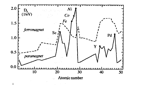
Figure 2.42. Stoner criterion for metallic elements: (full curve) \( \mathcal{D}_{\sigma}(E_{\text{F}})\) and (dashed curve) \(1/I\). There are only three elements exhibiting ferromagnetism; Sc, Y, and Pd are exchange-enhanced Pauli paramagnets.
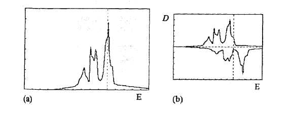
Figure 2.43. Density of states (DOS) for bcc iron: (a) paramagnetic DOS and (b) ferromagnetic DOS.
metals such as Sc and Pd are strongly exchange-enhanced Pauli paramagnets close to ferromagnetism. A more physical explanation is that the gain in Coulomb interaction energy has to compete against one-electron energies whose order of magnitude is given by the bandwidth. The ultimate reason for the ferromagnetism of the late 3d elements is their large density of states at \(E_{\text{F}}\). By comparison, the variation of the Stoner parameter \(I\) is of secondary importance.
There are several reasons for the large transition-metal DOS: (i) d bands have to accommodate 10 electrons per atom, as opposed to s bands, which contain only two electrons per atom; (ii) incompletely filled transition-metal electron shells lie well inside the atoms (table 2.15), so that the overlap of the 3d wavefunctions is small; (iii) across a given transition-metal series, there is a contraction of the
Table 2.15. Properties of partly filled shells of metallic elements. The atomic diameters are given for comparison (1 pm = 0.01 Å).
| Element | Atomic diameter (pm) | Shell diameter (pm) | Band width (eV) |
|---|---|---|---|
| Mn | 252 | 171 | 5.8 |
| Fe | 250 | 153 | 5.3 |
| Co | 251 | 138 | 4.8 |
| Ni | 250 | 127 | 3.9 |
| Pt | 277 | 225 | 7.0 |
| Gd | 335 | 108 | 0.3 |
Table 2.16. Intrinsic properties of the ferromagnetic 3d elements. \(m\) and \(M_{0}\) refer to zero temperature.
| \(m\) (\(\mu_{\text{B}}\)) | \(\mu_{0}M_{0}\) (T) | \(T_{\text{C}}\) (K) | \(D_{\text{s}}(E_{\text{F}})\) (eV-1) | \(I\) (eV) | |
|---|---|---|---|---|---|
| Fe | 2.23 | 2.22 | 1044 | 1.54 | 0.93 |
| Co | 1.73 | 1.85 | 1390 | 1.72 | 0.99 |
| Ni | 0.62 | 0.66 | 628 | 2.02 | 1.01 |
d shells caused by the increasing nuclear charge and (iv) often the DOS exhibits pronounced peaks at the Fermi level (figure 2.43). Some intrinsic properties of the ferromagnetic 3d elements are shown in table 2.16.
It is instructive to compare the Stoner theory with the ionic magnetism predicted by Hund's rules. The spin-dependent part of the one-electron potential favours maximum spin alignment and corresponds to Hund's first rule. Hund's third rule governing the relation between spin and orbital angular momenta is not included in (2.179), but it is easily incorporated into the independent-electron theory by adding a spin-orbit coupling term (section 2.1.3.6). Together with the crystal-field potential and the hopping energy, the spin-orbit coupling determines the anisotropy contribution of the itinerant 3d electrons (section 3.1.4). Finally, the one-electron potential may depend on the magnetic quantum number of the localized orbitals. This effect is known as orbital polarization (Severin et al 1993) and corresponds to Hund's second rule.
Weak and Strong Ferromagnetism
The Stoner criterion determines the existence of ferromagnetism but it cannot predict the magnitude of the magnetic moment. Minimization of the total energy (2.179) shows that the transfer of electrons from the \(\downarrow\) band to the \(\uparrow\) band
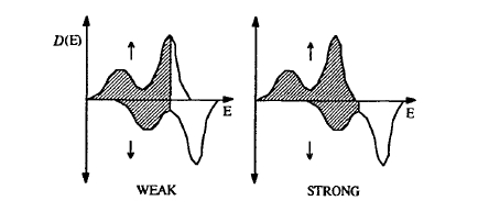
Figure 2.44. Weak and strong ferromagnetism (schematic).
Table 2.17. Filling of the \(\uparrow\) and \(\downarrow\) bands in elemental 3d metals.
| \(n_{3d} + n_{4s}\) | \(n_{3d}(\uparrow)\) | \(n_{3d}(\downarrow)\) | \(n_{4s}(\uparrow)\) | \(n_{4s}(\downarrow)\) | 3d\(\uparrow\) holes | 3d\(\downarrow\) holes | \(m/\mu_{\text{B}}\) | |
|---|---|---|---|---|---|---|---|---|
| Cr | 6 | 2.7 | 2.7 | 0.3 | 0.3 | 2.3 | 2.3 | 0 |
| Mn | 7 | 3.2 | 3.2 | 0.3 | 0.3 | 1.8 | 1.8 | 0 |
| Fe | 8 | 4.8 | 2.6 | 0.3 | 0.3 | 0.2 | 2.4 | 2.2 |
| Co | 9 | 5.0 | 3.3 | 0.35 | 0.35 | 0.0 | 1.7 | 1.7 |
| Ni | 10 | 5.0 | 4.4 | 0.3 | 0.3 | 0.0 | 0.6 | 0.6 |
| Cu | 11 | 5.0 | 5.0 | 0.5 | 0.5 | 2.3 | 2.3 | 0 |
The process continues until the Stoner exchange balances the increase in kinetic energy. The exchange splitting between the \(\uparrow\) and \(\downarrow\) bands is then given by \(\Delta E = Im/\mu_{\text{B}}\).
An important concept is the distinction between strong and weak ferromagnetism illustrated in figure 2.44. Cobalt and nickel are strong ferromagnets with fully polarized \(3d\uparrow\) subbands and partly filled \(3d\downarrow\) subbands. Iron, if it behaved similarly, would have a moment of about \(2.7 \mu_{\text{B}}\) and its magnetization would be \(\mu_{0}M_{0} = 2.8\) T. In fact, the atomic moment of \(2.22 \mu_{\text{B}}\) for iron indicates an incompletely polarized \(3d\uparrow\) subband, which is referred to as weak ferromagnetism. Table 2.17 illustrates this distinction by showing the \(3d\)-band occupancy or \(d\) count for some \(3d\) elements.
The moments of strong ferromagnets are easily estimated from \(d\)-count considerations, since adding or removing electrons, for instance by alloying, changes the number of \(\downarrow\) holes. As a rule, the \([Ar]3d^{n}4s^{2}\) configuration means that \(n\) \(3d\) electrons and, for late \(3d\) elements, about \(1.35\) \(4s\) electrons enter the \(3d\) band, because the upper part of the broad and nearly unpolarized \(4s\) band has a fairly high energy. There are ten \(3d\) states altogether, so that the assumption of a completely filled spin-up band yields \(n + 1.35 - 5\) spin-down electrons. Subtracting this number from the number \(5\) of spin-up electrons yields the moment \(m = (8.65 - n) \mu_{\text{B}}\), that is \(m \approx 1.65 \mu_{\text{B}}\) for cobalt and \(m \approx 0.65 \mu_{\text{B}}\) for nickel. This filling mechanism yields the descending branch of the Slater-Pauling curve, that is the full line in figure 2.45.
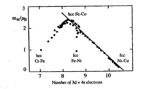
Figure 2.45. The Slater-Pauling curve showing the magnetic moments of some alloys having bcc (Fe-V, Fe-Cr, Fe-Mn, Fe-Co, Fe-Ni) or fee (Fe-Co, Fe-Ni, Ni-Co, Ni-Cu) structures. The full line indicates strong ferromagnetism.
Half-metallic ferromagnets are strong ferromagnets with no 4s states at the Fermi level. There is therefore a \(\uparrow\) DOS at \(E_{\text{F}}\), but a semiconductor-like \(\downarrow\) density of states (or vice versa). A few Heusler alloys such as MnNiSb and metallic oxides such as \(\text{CrO}_{2}\) (section 5.1), belong to this class. Like ionic compounds, stoichiometric half-metallic ferromagnets have a magnetic moment which is an integral number of Bohr magnetons per formula since \(n_{4s} = n_{3d\downarrow} = 0\).
Intermetallic Compounds
A generalization of the d-count approach is the magnetic valence approximation for strong ferromagnets (Holes et al 1983). The term magnetic valence indicates that spin-down holes are filled according to the chemical valence \(n\) of the atoms. In the case of binary alloys \(A_{1 - x}B_{x}\), one obtains the average magnetic moment \(m/\mu_{\text{B}} = (1 - x)m_{\text{A}}' + xm_{\text{B}}'\), where \(m_{\text{A}}'\) and \(m_{\text{B}}'\) describe the magnetic activity of the respective constituents. Typical values are \(m' = 8.65 - n\) for the late 3d elements and \(m' = 0.65 - n_{\text{v}}\) for metalloids, where \(n_{\text{v}}\) is the number of valence electrons. For instance, \(m' = 0.35\) for hydrogen in 3d metals. Note, however, that this particular approach does not apply to very electronegative elements such as nitrogen.
It is worth emphasizing that the magnetic-valence model is not a rigid-band model, because the local DOSs of neighbouring atoms modify each other. In particular, charge neutrality forbids inter-atomic electron transfer in metals, which is realized by screening and leads to a skewing of the DOS. As a matter of fact, since elemental densities of states do not superpose in alloys, it is often difficult to predict the magnetic moment from the atomic composition. For example, the ferromagnetism of substances such as \(\text{MnBi}\) (\(T_{\text{C}} = 630\) K), \(\text{CrO}_{2}\) (\(T_{\text{C}} = 396\) K) and \(\text{ZrZn}_{2}\) (\(T_{\text{C}} = 17\) K) indicates that the Stoner criterion
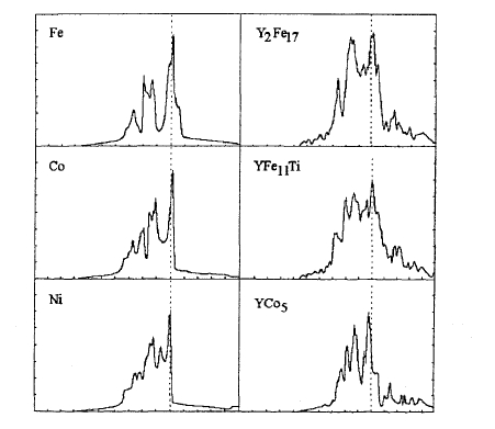
Figure 2.46. Typical paramagnetic densities of states.
may well be satisfied for compounds consisting entirely of non-ferromagnetic elements.
The highest room-temperature magnetization ever achieved in a material is \(\mu_{0}M_{\text{s}} = 2.43\) T in \(\text{Fe}_{65}\text{Co}_{35}\). Increasing the iron content beyond 65 at.% leads to weak ferromagnetism, which causes the moment to lie below the full line in figure \(2.45^{30}\). The high magnetization of \(\text{Fe}_{65}\text{Co}_{35}\) is exploited in alnico-type permanent magnets (section 5.2).
Since the magnetization of rare-earth permanent magnets is largely given by the transition-metal sublattice, it is useful to consider isostructural compounds containing non-magnetic rare earths such as yttrium. For instance, the iron-sublattice magnetization of \(\text{Nd}_{2}\text{Fe}_{14}\text{B}\) does not differ very much from that of \(\text{Y}_{2}\text{Fe}_{14}\text{B}\). Paramagnetic densities of states of some intermetallics relevant to permanent magnetism are shown in figure 2.46.
There is a general rule that the ferromagnetism of iron-rich alloys, such as \(\text{Sm}_{2}\text{Fe}_{17}\), is less stable than that of isostructural cobalt compounds. However, since the DOS is inversely proportional to the bandwidth, ferromagnetism is
30 An interesting material is the metastable nitride \(\alpha^{\prime}-\text{Fe}_{16}\text{N}_{2}\) (Jack 1951, Kim and Takahashi 1972), where bulk moments of about \(3\ \mu_{\text{B}}\) per iron atom have been claimed, but these findings have not been reproduced in the bulk.
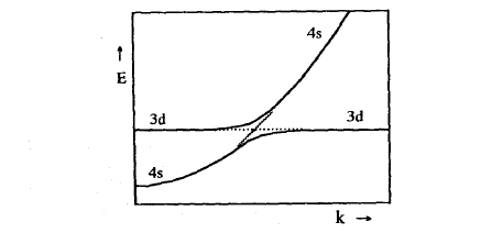
Figure 2.47. Wave-vector dependence of the hybridization between a broad s band and a very narrow d band.
stabilized by lattice expansion. A method to increase the lattice constants of intermetallic compounds is interstitial modification using atoms such as hydrogen, carbon and nitrogen. Nitrogen and carbon are better than hydrogen, since hydrogen electrons tend to occupy unoccupied 3d↓ states (Coey and Sun 1990, Coey 1996). A good example is the production of Sm2Fe17N3 by gas-phase interstitial modification. Among other positive effects, the moment of Sm2Fe17N3 is more stable than that of the unexpanded parent compound Sm2Fe17, and both moment and Curie temperature (section 2.4.3) are enhanced. Another example is (metastable) fcc iron, which is paramagnetic or antiferromagnetic at low inter-atomic distances but becomes ferromagnetic on lattice expansion, as found in Fe80Ni20.
Beyond the Tight-binding Stoner Theory
The conceptual simplicity of the 3d tight-binding approach does not mean that actual calculations are trivial. For example, Y2Fe14B has 56 iron atoms per unit cell and five 3d orbitals per atom, so that one has to diagonalize a 280×280 matrix for each k point. Besides these fairly demanding computational requirements, the tight-binding Stoner theory suffers from a number of more fundamental shortcomings.
Iron-series transition metals are characterized by a narrow 3d band which is embedded in a broad free-electron-like 4s band. Since the states at the top of the 4s band have a very high energy, some of the 4s electrons enter the 3d band and modify the 3d magnetic moment. Furthermore, the hybridization between the two bands (s–d mixing) shown in figure 2.47 yields a small polarization of the 4s band. This means that a more general version of the tight-binding approach has to consider at least six orbitals per atom, regardless of the question of whether a tight-binding description of the nearly-free 4s electrons is physically reasonable.
A difficult problem is the choice of the one-electron potential \(V(\mathbf{r})\). In the tight-binding approximation, the potential is parametrized in terms of hopping integrals and on-site energies, but in general it is a non-local Hartree–Fock functional of the electron density which has to be determined self-consistently. Due to the complexity of exact one-electron calculations it is common to use the local-density approximation, where real correlations are replaced by the free-electron correlations of a dense electron gas. In particular, (2.158) and \(k_{\text{F}} = (3\pi^{2}N/\Omega)^{1/3}\) imply that the local exchange potential scales as \(n(\mathbf{r})^{1/3}\). Furthermore, since the exchange splitting modifies the shape of the \(\uparrow\) and \(\downarrow\) subbands (figure 2.43) it is necessary to consider spin-dependent potentials \(V_{\sigma}(\mathbf{r})\). A simple example is the model (2.108), where \(V_{\pm}(\mathbf{R}_{i}) = \pm V_{0}(\mathbf{R}_{i})\).
There are various self-consistent and non-self-consistent methods to calculate the band structure of transition metals. For example, self-consistent augmented spherical wave (ASW) calculations were used to calculate the band structures of \(Y_{2}Fe_{17}\), \(Y_{6}Fe_{23}\), \(YFe_{2}\) and \(YFe_{3}\) (Coehoorn 1989). Local spin-density approximation band-structure calculations are able to predict the observed moments in 3d metals and alloys with an exactness of about 5%. Note, however, that reasonable moment predictions do not necessarily prove the quality of an approximation. The point is that the magnetic energy is a highly nonlinear function of the magnetization (figure 2.37), so that a barely satisfied Stoner criterion may be sufficient to assure nearly complete spin polarization of the d band.
In section 2.1.6 we have seen that one-electron (independent-electron) calculations exaggerate the tendency towards ferromagnetism. The ultimate reason is the mean-field character of the one-electron approach31. Mathematically, the one-electron approach amounts to the calculation of Hartree–Fock energies from a single Slater determinant, whereas many-body approaches such as the configuration interaction method (CI) involve two or more Slater determinants. Interestingly, some aspects of correlation are contained in unrestricted Hartree–Fock calculations, where one-electron wavefunctions are used that have a lower symmetry than the starting Hamiltonian. In some sense, spin-dependent band-structure calculations and models such as (2.108) can be interpreted as unrestricted Hartree–Fock approaches.
A feature of the time-dependent Schrödinger equation is that energy differences can be interpreted as transition frequencies \(\omega = \Delta E/\hbar\). As a consequence, narrow and broad bands indicate slow and fast inter-atomic hopping, respectively. This has a great impact on the behaviour of d electrons in metals. Consider, for example, the hopping transition \(3d^{9} + 3d^{9} \rightarrow 3d^{8} + 3d^{10}\), which gives rise to atomic charges \(\pm e\). Since the hopping frequency of 4s electrons is much larger than that of 3d electrons, the charge differences will be
31 This trend is not restricted to zero-temperature many-body interactions but also applies to finite-temperature magnetism. For example, mean-field theory predicts the paramagnetic one-dimensional Ising model to be ferromagnetic.
screened nearly instantaneously by 4s electrons. This mechanism reduces the value of the Coulomb interaction \(U \approx 10\ \text{eV}\) by an order of magnitude and \(U\) is normally treated as an adjustable parameter.
As a rule, metals containing light actinides such as uranium exhibit delocalized 5f magnetism. However, the comparatively strong actinide spin-orbit coupling means that 5f orbital moments are much less quenched than 3d orbital moments. For example, the zero-temperature moment \(1.55\ \mu_{\text{B}}\) of US (\(T_{\text{C}} = 177\ \text{K}\)) originates from spin and orbital moments of about \(+3.5\ \mu_{\text{B}}\) and \(-2\ \mu_{\text{B}}\), respectively. By comparison, 3d orbital-moment contributions are of the order of \(\pm 0.1\ \mu_{\text{B}}\). Note that spin-orbit coupling in itinerant magnets not only produces an orbital moment but also yields magnetocrystalline anisotropy (section 3.1.2).
Spin Fluctuations in Magnetism
A shortcoming of the Stoner theory is that it greatly overestimates the ferromagnetic ordering temperature of itinerant magnets. Furthermore, it predicts a Pauli paramagnetic susceptibility above the ordering temperature, whereas most itinerant ferromagnets exhibit a Curie–Weiss-like susceptibility. Thermally activated electron transfer from \(\uparrow\) to \(\downarrow\) states reduces the magnetization and destroys the itinerant magnetic moment above the Stoner temperature \(T_{\text{S}}\), but in general the \(T_{\text{S}}\) is much higher than the Curie temperature. For example, the assumption of a single dominating peak in the density of states leads to \(k_{\text{B}}T_{\text{S}} = mI/4 \mu_{\text{B}}\), that is \(T_{\text{S}} \approx 2900\) K for iron, whereas the Stoner temperature is around \(4000\) K for Co and \(2600\) K for Ni.
The failure of finite-temperature Stoner theory is due to the assumption of Bloch wavefunctions (2.161). The delocalized character of Bloch wavefunctions implies that moment and spontaneous magnetization vanish simultaneously at the Stoner temperature. This is unrealistic. In reality, short-wavelength excitations are able to destroy the magnetization far below \(T_{\text{S}}\). Conversely, specific-heat and susceptibility measurements and neutron-scattering experiments show that a part of the itinerant moment survives at and above \(T_{\text{C}}\). This spin-fluctuation behaviour means that the behaviour of itinerant magnets is intermediate between the Heisenberg and Stoner approaches. At \(T_{\text{C}}\), the moment is only partly reduced, but the magnetization direction fluctuates as in local-moment magnets. In other words, the electrons stay for most of the time on individual atomic sites where on-site correlations dominate.
Depending on how close metallic ferromagnetism is to the Stoner theory one can establish two limits. The finite-temperature behaviour of very weak itinerant ferromagnets is determined by long-wavelength spin fluctuations close to the Stoner limit. In strong and nearly strong ferromagnets, such as Co, bcc Fe and Sm2Fe17N3, short-wavelength spin fluctuations are important and the moment is only slightly reduced at \(T_{\text{C}}\).
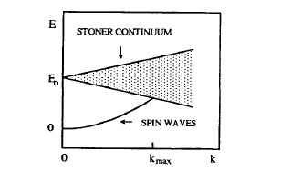
Figure 2.48. Excitations in itinerant ferromagnets (see e.g. Thompson 1965). Since \(E_{0}\) can be interpreted as the exchange splitting \(Im\), \(k_{\text{max}}\) is small for very weak itinerant ferromagnets.
Quantum Statistics
A systematic analysis of spin excitations such as spin waves and Stoner excitations (figure 2.48) is based on many-body quantum statistics. A major problem is that the partition function \( \mathcal{Z} = \text{Tr}(\exp(-\hat{T}/k_{\text{B}}T))\) contains quadratic operator products such as the Hubbard interaction term \(\hat{n}_{i\uparrow}\hat{n}_{i\downarrow}\) (section 2.1.6, section 2.4.2.2). There are several methods to cope with this problem. To remove quadratic operator expressions from the Boltzmann exponent one can use the Hubbard-Stratonovich transformation
\(\text{e}^{-\hat{u}^{2}} = \int_{-\infty}^{\infty} \text{e}^{-\pi x^{2}} \text{e}^{-2i(\pi)^{1/2}x\hat{u}} \text{d}x\). (2.182)
This simplification is paid for by the introduction of a fictitious random field \(x\), which may be interpreted as thermal disorder. Furthermore, the evaluation of the Gaussian average is very difficult since the operators involved do not commute. On a mean-field level it is possible to map the problem onto the Schrödinger equation for the motion of an electron in a spin and temperature dependent exchange field. A very simple example is the model (2.108) if we interpret the matrices \((a)\) and \((b)\) as ground-state and finite-temperature potentials, respectively. Since the evaluation of exact quantum-statistical expressions, such as (2.182), is very complicated, we will now focus on simple statistical models.
Very Weak Itinerant Ferromagnets
These materials are characterized by a small zero-temperature moment, \(m < 0.1\ \mu_{\text{B}}\) per formula unit. A quasi-classical theory which describes long-wavelength spin fluctuations in very weak itinerant ferromagnets is the
>self-consistent renormalization of spin fluctuations32. The starting point is the Hamiltonian
\(\mathcal{H} = \int [A(\nabla s(\mathbf{r}))^{2} + \eta(s)] \text{d}\mathbf{r}\) (2.183)
where the magnetic energy is, to a fair approximation, given by the double-well potential
\(\eta(s) = -\frac{1}{2}as^{2}(\mathbf{r}) + \frac{1}{4}bs^{4}(\mathbf{r})\). (2.184)
To obtain an analytic expression for the partition function we have to replace the energy density \(\eta\) by an approximate quadratic expression \(\eta = a_{\text{eff}}s^{2}/2\). Interpreting this quadratic term as a trial energy (see appendix A4.3) one obtains
\(a_{\text{eff}} = a - 3\langle s^{4}\rangle b\). (2.185a)
In other words, aside from a prefactor the term \(s^{4}\) is approximated by \(\langle s^{2}\rangle^{2}\).
Using \(a_{\text{eff}}\), the partition function \(\mathcal{Z} = \int \exp(-\mathcal{H}/k_{\text{B}}T) \text{d}s\) and quantities such as the susceptibility \(\chi\) can be calculated without further approximations. Taking into account the fact that \(\chi\) diverges at the Curie temperature one obtains
\(T_{\text{C}} = \frac{2\pi^{2} A a}{3 b k_{\text{B}} k_{0}}\). (2.186)
Here \(k_{0} \approx k_{\text{max}}\) is a short-wavelength cut-off wavevector below which excitations contribute to the breakdown of the magnetization at \(T_{\text{C}}\) (figure 2.48). In the delocalized limit, \(k_{0}\) is much smaller than the inverse lattice spacing, so that \(T_{\text{C}}\) approaches the high Stoner temperature.
The Limit of Large Spin Polarization
Since not only strong ferromagnets such as Co but also weak ferromagnets such as Y2Fe17 exhibit a large exchange splitting, the materials of interest here cannot be described in terms of the Murata-Doniach theory. For example, replacing (2.184) by a more accurate magnetic energy \(\eta(s)\) derived from band-structure calculations yields
\(a_{\text{eff}} = \frac{(2\pi)^{-1/2}}{\langle s^{2}\rangle^{5/2}} \int_{-\infty}^{\infty} \{s^{2} - \langle s^{2}\rangle\} \eta(s) \text{e}^{-s^{2}/(2\langle s^{2}\rangle)} \text{d}s\). (2.185b)
Real materials are characterized by an upper limit \(s_{\text{max}}\) to the spin variable, since the spin polarization cannot go beyond complete exchange splitting. This implies \(\eta(s) = \infty\) for \(|s| > s_{\text{max}}\) and leads to the unphysical results \(a_{\text{eff}} = \infty\) and \(T_{\text{C}} = 0\).
32 This approach (Murata and Doniach 1972) is also known as phenomenological mode-mode coupling theory or the classical utilizer-integral method. By comparison, quantum-mechanical functional integral approaches utilize equations such as (2.182).
Another aspect of the problem is that Hartree–Fock exchange constants such as (2.57) contain both intra-atomic (U) and inter-atomic (J) contributions. In local-moment magnets, J and U are responsible for magnetic order and moment formation, but this separation is less pronounced in itinerant magnets. Consider the simple quasi-classical model Hamiltonian
\(\mathcal{H} = -z\mathcal{J}_{0}(s) \cdot s - \left(1 - \frac{1}{\mathcal{D}(E_{\text{F}})}\right) s^{2}\) (2.187)
where the inter-atomic exchange is parametrized by a classical mean-field Heisenberg exchange constant \(\mathcal{J}_{0} \ll I - \mathcal{D}(E_{\text{F}})\). The \(s^{2}\) Stoner term describes the moment formation due to intra-atomic exchange (I). Figure 2.37 shows that, by definition, the squared spin polarization \(s^{2} \leq 1^{33}\). Zero-temperature ferromagnetism is characterized by \(s = \pm 1\), but at finite temperatures both the magnetization (s) and the squared magnetization (\(s^{2}\)) are reduced by Heisenberg and Stoner excitations, respectively. The Stoner contribution is important when \(I - \mathcal{D}(E_{\text{F}})\) is small, that is when the Stoner criterion is only barely satisfied.
Putting \(s^{2} = 2s(s)\) in (2.187) is equivalent to extending the mean-field approximation to the magnetic moment and yields the Stoner-type Curie temperature
\(T_{\text{C}} = \frac{1}{6k_{\text{B}}} \left(I + 2z\mathcal{J}_{0} - \frac{1}{\mathcal{D}(E_{\text{F}})}\right)\). (2.188)
Like (2.57), this equation is unable to distinguish between intra- and inter-atomic exchange and yields Curie temperatures which are much too high. By comparison, the appropriate solution of (2.187) is34
\(T_{\text{C}} = \frac{z\mathcal{J}_{0}}{3k_{\text{B}}} \left(1 - \frac{1}{3\left(I - 1/\mathcal{D}(E_{\text{F}})\right)}\right)\). (2.189)
In this equation, the intra-atomic exchange (I) and the inter-atomic hopping (1/D) yield a small correction to the local-moment Curie temperature \(z\mathcal{J}_{0}/3k_{\text{B}}\) (for a somewhat simplistic explicit model calculation see appendix A4.3).
Many iron-rich alloys exhibit Curie temperatures which are much lower than those of their isostructural cobalt alloys (section 5.3). This is of direct relevance in permanent magnetism, because it excludes rare-earth iron magnets from high-temperature applications. A simplistic explanation is that exchange integrals are negative and positive for the small and large inter-atomic distances, respectively, as suggested by the Bethe–Slater–Néel curve (figure 2.8). Equation (2.50b) shows that direct exchange integrals are always positive, but (2.57), (2.107) and the model (2.108) show that effective inter-atomic exchange constants are modified by inter-atomic hopping and may be negative. On the other hand, (2.189) predicts a strong Curie-temperature reduction when the Stoner criterion
33 The quadratic dependence of the magnetic energy on s amounts to a rectangular DOS.
34 This result is obtained by using \(k_{\text{B}}T_{\text{C}} = z\mathcal{J}_{0}(s(T_{\text{C}}))/3\) and taking into account the fact that \(s(T_{\text{C}})\) is not much smaller than one in the considered limit.
is barely satisfied. From figure 2.40 we see that the paramagnetic density of states at the Fermi level is rather low for fcc Fe, as opposed to bcc Fe, fcc Co and fcc Ni35. This weakens the trend towards ferromagnetism in fcc Fe and other dense-packed iron-rich intermetallics, where there are closed three-hop nearest-neighbour loops in the moments expansion. Furthermore, the large number of non-equivalent crystallographic sites leads to a splitting of the DOS main peak into numerous subpeaks, which reduces the maximum height of the main peak and contributes to the Curie-temperature reduction.


