

4. Experimental Methods: Techniques for Exploring Magnetism
Experiments provide the quantitative information about materials properties on which all applications depend. They also serve to inspire and refine physical theory. The traditional image of apparatus on a laboratory bench has evolved so that some measurements are now conducted at national or multinational institutes built around large - scale facilities for generating high magnetic fields, neutron beams or intense streams of UV or x - ray radiation. Meanwhile, computers have evolved in the opposite sense, from central facilities to benchtop instruments for data acquisition, modelling and visual display of results. Numerical computations and simulations may be regarded as an experimental tool for investigating a model reality where complex magnetic behaviour at the atomic, micromagnetic and system levels can be investigated with the aid of a workstation. Magnetism nevertheless remains a science based on regular recourse to the touchstone of measurement.
Here we give a brief account of the experimental methods used to investigate magnetism, first at the atomic level, then at the macroscopic level and finally for examining permanent magnets at the system level.
Atomic-Scale Magnetism: Unlocking the Secrets of Magnetic Materials
The foundation of magnetism in solids is the atomic - scale structure of the crystal. The electronic structure of the atoms, together with the crystal (or amorphous) structure of the solid, determine atomic moments, exchange and dipolar interactions and crystal fields which are the ingredients of collective magnetic order. Direct imaging of individual magnetic atoms is at the extreme limit of current experimental capabilities. Instead, the main methods used to probe the intrinsic magnetic properties are diffraction and spectroscopy, respectively the elastic and inelastic scattering by the solid of a beam of particles or electromagnetic radiation. If the wavevector and energy of the incident and scattered beams are \((\boldsymbol{K},h\Omega)\) and \((\boldsymbol{K}',h\Omega')\), complete information about the
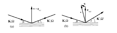
Figure 4.1. Scattering of a beam of radiation from a crystal. (a) Elastic scattering in the Bragg geometry where \(\boldsymbol{K}-\boldsymbol{K}'=\boldsymbol{g}_{hkl}\); (b) inelastic scattering in the vicinity of a Bragg peak, where \(\boldsymbol{K}-\boldsymbol{K}'=\boldsymbol{g}_{hkl}+\boldsymbol{q}\)
The differential scattering cross - section of a solid is contained in the differential scattering cross - section
\(\sigma_{\mathrm{dif}}=\mathrm{d}^{2}\sigma(\boldsymbol{\kappa},\omega,T)/\mathrm{d}\kappa\mathrm{d}\omega\) (4.1)
where \(\sigma\) is the integral cross - section from zero to \(\kappa\) and \(\omega\) and where \(|\boldsymbol{\kappa}| = |\boldsymbol{K}-\boldsymbol{K}'|\), \(\omega=\Omega'-\Omega\) (figure 4.1). Commonly used particle beams are neutrons and electrons. With electromagnetic radiation such as x - rays the polarization is another relevant variable. Sometimes it is possible to detect directly the scattered radiation. In other cases, such as Auger electron spectroscopy or electron in photoemission spectroscopy, and also analyse the spins of the incident and scattered or excited particles. Different experimental methods probe different aspects of the generalized susceptibility. They provide a description of the crystal and magnetic structure, the electronic structure and the distribution of spin and orbital moments. The inter - atomic exchange and crystal - field parameters can be determined. Further understanding of the electronic structure is provided by computational methods.
Structure: Investigating the Atomic Arrangement in Magnetic Materials
Diffraction methods are used to study both the crystal structures and magnetic structures of solids. A beam of radiation is needed whose wavelength is comparable to the inter – atomic spacing (about 200 pm [2Å]). The radiation is scattered by the atomic electrons or nuclei or, in the case of neutrons, by the magnetic moments of the electrons. Interference of the scattered waves gives rise to a number of diffracted beams in precisely defined directions relative to the crystal axes. Directions of these Bragg reflections are determined by the lattice parameters, according to Bragg’s law
\(2d_{hkl}\sin\theta = n\lambda\) (4.2)
where \(d_{hkl}\) is the spacing of a set of reflection planes whose Miller indices are \((h,k,l)\). Both incident and diffracted beams make an angle \(\theta\) with the \(hkl\) planes, as shown in figure 4.1. The scattering is elastic so that \(|\boldsymbol{K}| = |\boldsymbol{K}'|\) and the scattering vector \(\boldsymbol{\kappa}\) is perpendicular to the reflecting planes. The wavelength
of the radiation \(\lambda = 2\pi/K\) and the integer \(n\) is known as the order of the reflection. The Bragg condition is equivalent to the requirement that \(\boldsymbol{\kappa}\) is a reciprocal lattice vector \(\boldsymbol{g}_{hkl}=2\pi\boldsymbol{r}_{hkl}/d_{hkl}\). Conventionally, the integer \(n\) is absorbed into the definition of the Miller indices \((h,k,l)\). Relations between the lattice parameters \(a,b,c\) and the spacings of the \(hkl\) planes are \(d_{hkl}^{-2}=h^{2}/a^{2}+k^{2}/b^{2}+l^{2}/c^{2}\) for any crystal system with orthogonal axes and \(d_{hkl}^{-2}=\{(4/3)(h^{2}+hk + k^{2})+l^{2}/c^{2}\}c^{-2}\) for the hexagonal system1. Intensities of the Bragg reflections depend on the strength of the atomic scattering and the disposition of atoms within the unit cell. They are proportional to the square of the complex structure factor
\(F_{hkl}=\sum_{i}f_{i}\exp(-\mathrm{i}\boldsymbol{\kappa}\cdot\boldsymbol{r}_{i})=\sum_{i}f_{i}\exp[-2\pi\mathrm{i}(h x_{i}+k y_{i}+l z_{i})]\) (4.3a)
where the sum is over all the atoms at positions \(\boldsymbol{r}_{i}=x_{i}\boldsymbol{a}+y_{i}\boldsymbol{b}+z_{i}\boldsymbol{c}\) in the unit cell, \(f_{i}\) is the atomic scattering factor, which has dimensions of length and generally depends on \(\boldsymbol{\kappa}\) or \(\theta\). Coherent scattering of the Bragg peaks and their inelastic satellites is produced by constructive interference of waves scattered from different atomic sites as distinguished from incoherent scattering which arises when there is phase relaxation between waves scattered from different sites and no constructive interference.
X - ray Diffraction
This is the standard method of crystal structure analysis. The energy \(E = h\Omega=hc/\lambda\) of electromagnetic radiation associated with a wavelength of 200 pm is 6.20 keV, which is close to the K absorption edge for Cr. The K edge corresponds to the energy needed to ionize an atom by creating a K - hole. The L edges correspond to 2s or 2p hole s. In a laboratory x - ray set, a target of a suitable metal in a sealed tube is bombarded with energetic electrons. Characteristic x - ray radiation is emitted as electrons from outer shells de - excite to fill holes created in the inner shells (figure 4.2a). The flux from a sealed tube is typically \(10^{10}\) photons per second. The K edge for the commonly used copper target, for example, is at 8.98 keV and nearly monochromatic \(K_{\alpha}\) radiation with \(\lambda = 0.1542\ nm\) is produced as holes in the Is shells are filled by 2p electrons. \(K_{\beta}\) radiation is produced when the 1s shells are filled by 3p electrons.
X - rays are scattered by the charge of the atomic electrons, and the appropriate atomic scattering function in equation (4.3b) is proportional to the Fourier transform of the atomic charge distribution \(\rho(\boldsymbol{r})\):
\(f(\boldsymbol{\kappa})=\int_{\mathrm{c}}\rho(\boldsymbol{r})\exp(-\mathrm{i}\boldsymbol{\kappa}\cdot\boldsymbol{r})\mathrm{d}\boldsymbol{r}=Zf_{\mathrm{j}}(\boldsymbol{\kappa})\). (4.3b)
1 Rhombohedral crystals are often indexed on a hexagonal cell.
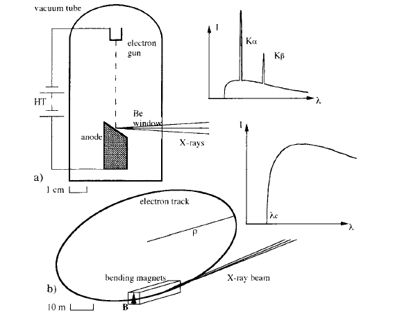
Figure 4.2. Sources of x - rays: (a) a sealed laboratory x - ray tube; (b) a synchrotron source. The intensity from a synchrotron is more than four orders of magnitude greater than from an x - ray tube.
Here \(Z\) is the atomic number, \(f_{\mathrm{X}}(0)=1\) and \(r_{\mathrm{e}}\) is the electron'readius', the scattering length for an electron; its value, \(\mu_{0}e^{2}/4\pi m_{\mathrm{e}} = 2.818\ fm\).
Samples for investigation by x - ray or neutron diffraction are often in powder form. Randomly oriented crystallite powder scatters the incident monochromatic beam in a series of cones centred on the incident beam axis; each cone corresponds to a Bragg reflection from a set of randomly oriented crystallites. A point detector or linear multidetector is then used to measure the diffraction intensity as a function of \(2\theta\) in the scattering plane. A typical diffraction pattern for an \(\text{SmCo}_{5}\) powder is shown in figure 4.3(a). Particle alignment restricts the diffracted beams to certain directions in the cones; for example if the \(c\) - axis is well aligned parallel to \(\boldsymbol{\kappa}\) as in the sintered \(\text{SmCo}_{5}\) magnet of figure 4.3(b), then the \(00l\) Bragg reflections dominate the powder pattern.
Far more intense fluxes of x - rays and UV radiation are available at synchrotron sources, where a beam of electrons or positrons is accelerated to a velocity close to that of light and then constrained by a magnetic field \(B\leq1\ T\) to travel around a storage ring which may be tens or hundreds of metres in diameter. The electron energy is typically \(5\ GeV\) or \(\gamma m_{\mathrm{e}}c^{2}\) with \(\gamma\approx10^{4}\). As they race around their track, the electrons emit a narrow beam of white
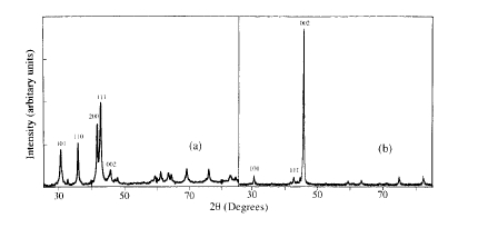
Figure 4.3. X - ray powder diffraction patterns from (a) a \(\text{SmCo}_{5}\) powder and (b) a sintered \(\text{SmCo}_{5}\) magnet with \(c\parallel\boldsymbol{\kappa}\)
radiation of width \((1 / \gamma_{\mathrm{e}})\) radians which is linearly polarized (more than 90%) in the plane of the orbit. The cut - off wavelength is \(4\pi\rho/3\gamma_{\mathrm{e}}^{3}=0.00714/B^{2}m_{\mathrm{e}}c\), where \(\rho\) is the radius of the electron orbit. Elliptically polarized radiation can be obtained by moving an entrance slit to collect radiation emitted just above or just below the orbit plane. Otherwise, circularly polarized radiation may be obtained using a wiggler or undulator insertion device of the type described in section 6.2.2. The energy of the x - rays is selected using x - ray mirrors and single - crystal monochromators. The huge photon fluxes of about \(10^{17}\) photons per second in a tightly collimated beam with a 0.1% energy bandwidth and high degree of polarization make synchrotron radiation very suitable for both absorption and photoelectron spectroscopy. Chemical selectivity is achieved by tuning the radiation to the appropriate atomic absorption edge.
Magnetic scattering of x - rays is typically smaller than charge scattering by a factor of \(10^{-5}\), making it impracticable to observe magnetic structures using sealed x - ray tubes. However, in the vicinity of an absorption edge the effect amounts to about 1% of the charge scattering which allows tunable synchrotron sources to be used for magnetic structure determination. The method is particularly useful for rare earths like Sm and Gd where neutron diffraction is hampered by an enormous neutron capture cross - section (table 4.1).
Neutron Diffraction
Neutron diffraction is the standard method for magnetic structure analysis. The neutron is an uncharged particle with spin \(1/2\) which carries a magnetic moment of \(- 1.91\ \mu_{\mathrm{n}}\), the nuclear magneton \(\mu_{\mathrm{n}} = 5.05\times10^{-27}\ A\ m^{2}\), which is smaller than the Bohr magneton by the ratio of the electron to the proton mass. Beams of neutrons are produced in specially optimized nuclear reactors
Table 4.1. Some nuclear (\(b\)) and magnetic (\(p\)) neutron scattering lengths in fm (\(10^{-15}\ m\)) and absorption cross - sections (\(\sigma_{\mathrm{a}}\)) in barns (\(10^{-28}\ m^{2}\)). All magnetic scattering lengths are for 3 - free ions, except for Ti - Fe, which are for spin - only \(3^{+}\) ions and Co - Ni which are for spin - only \(2^{+}\) ions.
| \(b\) | \(p(0)\) | \(\sigma_{\mathrm{a}}\) | \(b\) | \(p(0)\) | \(\sigma_{\mathrm{a}}\) | \(b\) | \(\sigma_{\mathrm{a}}\) | |||
|---|---|---|---|---|---|---|---|---|---|---|
| Ti | −3.4 | 2.7 | 6.1 | Y | 7.8 | — | 1.3 | B | 5.3 | 767 |
| V | −0.4 | 5.4 | 5.1 | Pr | 4.6 | 8.6 | 11.5 | C | 6.6 | 0.004 |
| Cr | 3.6 | 8.1 | 3.1 | Nd | 7.2 | 8.8 | 51.2 | N | 9.3 | 1.9 |
| Mn | −3.7 | 10.8 | 13.3 | Sm | 0.0 | 1.9 | 5670 | O | 5.8 | 0.0002 |
| Fe | 9.5 | 13.5 | 2.6 | Gd | 9.5 | 18.9 | 29400 | Al | 3.4 | 2 |
| Co | 2.5 | 8.1 | 37.2 | Tb | 7.4 | 24.3 | 23 | Si | 4.1 | 0.0 |
| Ni | 10.3 | 5.4 | 4.5 | Dy | 16.9 | 27.0 | 940 | Ti | 7.0 | 1.3 |
| Cu | 7.7 | 2.7 | 3.8 | Ho | 8.0 | 27.0 | 65 | Ba | 5.1 | 1.2 |
or in spallation sources where pulses of GeV protons from a linear accelerator produce bursts of neutrons as they impact on a heavy - metal target. The neutron energy for a de Broglie wavelength \(\lambda\) of 200 pm is \(h^{2}/2m_{\mathrm{n}}\lambda^{2}=0.0204\ eV\), which is comparable to \(k_{\mathrm{B}}T\) at ambient temperature. The neutrons from a reactor are thermalized in a moderator and a narrow slice is selected from the Maxwellian energy distribution by Bragg reflection from a single - crystal monochromator. Typical reactor fluxes are \(10^{15}\ cm^{-2}\ s^{-1}\), which have to be collimated and then reduced by two to three orders of magnitude by the monochromator. Monochromatic neutron beams from a high - flux reactor are roughly a thousand times weaker than monochromatic x - ray beams from a laboratory x - ray tube.
The scattering of thermal neutrons by an atomic nucleus is isotropic because nuclear interactions are very short - ranged; for an incident neutron plane wave \(\mathrm{e}^{\mathrm{i}\boldsymbol{k}\cdot\boldsymbol{r}}\), the scattered spherical wave \(\psi=-(b/r)\mathrm{e}^{\mathrm{i}kr}\) where \(b\) is the scattered length of the nucleus. In fact \(b\) is different for each isotope, so the values quoted for the elements in table 4.1 are isotopic averages. The scattering cross - section \(\sigma_{\mathrm{s}}\) is \(4\pi b^{2}\). Unlike x - ray scattering, where the scattering length increases as \(Z\), the number of atomic electrons, \(b\) varies erratically across the periodic table and can even change sign, which makes it possible to distinguish elements with similar atomic numbers.
The neutron is also scattered by the unpaired spin density of an atom. A magnetic scattering length \(p\) is defined as \((1.91r_{\mathrm{e}})Sf_{\mathrm{s}}\) for a spin - only moment. The quantity \(p\) is brackets is 5.4 fm. When both spin and orbital moments are present, \(p=(1.91r_{\mathrm{e}})Sf_{\mathrm{s}}+(1/2)Lf_{\mathrm{l}}\), where \(f_{\mathrm{s}}\) and \(f_{\mathrm{l}}\) are given by \([J(J + 1)\pm[S(S + 1)-L(L + 1)]]/[2J(J + 1)]\). The form factors \(f_{\mathrm{s}}\) and \(f_{\mathrm{l}}\) are normalized to unity at \(\theta = 0\). A magnetic interaction vector \(\boldsymbol{\mu}\) is defined as \(\boldsymbol{\mu}_{\mathrm{n}}=\boldsymbol{\mu}(\boldsymbol{\kappa}\cdot\boldsymbol{e}_{\mathrm{n}})/\kappa^{2}\) where \(\boldsymbol{e}_{\mathrm{n}}\) is a unit vector in the direction of the magnetic moment. For unpolarized neutrons, the intensities of the magnetic and nuclear
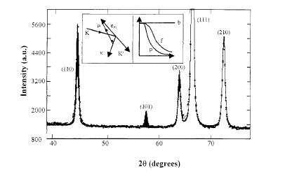
Figure 4.4. The neutron powder diffraction pattern for \(CrO_{2}\). Magnetic contributions to the Bragg peaks are shaded. The insets show the definition of the magnetic interaction vector \(\boldsymbol{\mu}\) and a comparison of the normalized atomic scattering factors for neutrons \((b, p)\) and x - rays \((f)\).
scattering add, so
\(\left|F_{hkl}\right|^{2}=\left|\sum_{i}b_{i}\exp(-\mathrm{i}\boldsymbol{\kappa}\cdot\boldsymbol{r}_{i})\right|^{2}+\left|\sum_{i}p_{i}\boldsymbol{\mu}_{i}\exp(-\mathrm{i}\boldsymbol{\kappa}\cdot\boldsymbol{r}_{i})\right|^{2}\) (4.4)
whereas if the neutron beam is polarized with magnetic moment in a direction \(\boldsymbol{\lambda}\) the intensity is
\(\left|F_{hkl}\right|^{2}=\left|\sum_{i}\{b_{i}+(\boldsymbol{\lambda}\cdot\boldsymbol{\mu}_{i})p_{i}\}\exp(-\mathrm{i}\boldsymbol{\kappa}\cdot\boldsymbol{r}_{i})\right|^{2}\). (4.5)
Since magnetic scattering depends on the orientation of the moments relative to the scattering vector, the complete magnetic structure (magnitudes and directions of the moments in a unit cell) can in principle be determined from the positions and intensities of the magnetic Bragg reflections. Note that there is no magnetic intensity when \(\boldsymbol{e}_{\mathrm{m}}\parallel\boldsymbol{\kappa}\).
A typical neutron powder diffraction pattern is shown in figure 4.4, together with the least - squares fit, to the theoretical Rietveld profile based on the unit cell parameters and scattering lengths. With large unit cells containing \(n\) atoms there can be as many as \(6(n + 1)\) structural and magnetic parameters to refine. Powder data are inadequate for structures more complex than that of \(Nd_{2}Fe_{14}B\) because of the limited number of Bragg reflections, and then one has to resort to single crystals and polarized neutrons. Some neutron scattering lengths and absorption cross - sections are listed in table 4.1.
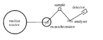
Figure 4.5. A triple-axis neutron spectrometer.
Spectroscopy: Probing Magnetic Properties at the Atomic Level
Many spectroscopic techniques are available to probe the energy levels and excitations of magnetic solids. Inelastic neutron scattering, where the energy and \(K -\)vector of an inelastically scattered beam are analysed, is the most general method because the changes both in energy and momentum of the neutron due to thermal excitations are appreciable. A triple - axis spectrometer (figure 4.5) is often used to measure \(q\) and \(\omega\). The spin - wave dispersion relations \(\omega(q)\) are measured by scanning the instrument near a Bragg peak to collect neutrons at constant energy or constant momentum transfer. The exchange constants \(\mathcal{J}_{ij}\) in the Heisenberg Hamiltonian for different pairs of interacting neighbours are deduced by fitting the dispersion curves. Dispersionless excitations such as crystal - field excitations of the rare - earth atoms can also be studied by inelastic neutron scattering.
Absorption spectroscopy and photoelectron spectroscopy can probe the structure of both valence and core electrons. The sample is irradiated with monochromatic photons of optical, UV or x - ray energies and either the transmitted beam or the ejected photoelectrons are analysed (figure 4.6). When the photoelectrons arise from core levels, the process is the inverse of x - ray generation. Photoemission is a surface - sensitive technique because the electrons can only emerge from a surface layer about 1 nm thick.
New methods depend on the availability of intense polarized light beams from synchrotron sources, and the ability to analyse the polarization of the transmitted photons or the spin of the ejected photoelectron. Angular - resolved UV photoelectron can give information on the spin - polarized density of states near the Fermi level \(E_{\mathrm{F}}\). The x - ray methods are element specific because the incident wavelength can be tuned to a desired absorption edge and the core levels of different elements do not usually overlap. X - ray absorption fine structure (EXAFS) observed near the absorption edge is a type of diffraction pattern produced by interference of the outgoing and backscattered electron waves. It gives information about the local environment of the absorbing atom, including coordination number and nearest - neighbour distances. Magnetic circular dichroism refers to the difference in the absorptive
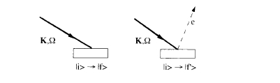
Figure 4.6. Absorption and photoemission processes for a single photon.
part of the refractive index of a solid for left - and right - circular polarized light passing through a sample magnetized parallel to \(\boldsymbol{K}\). For example, the 2p electrons of a transition element acquire an orbital moment from the helicity of the light as they are excited to unoccupied states just above the Fermi level and the absorption is governed by the density of unoccupied \(\uparrow\) and \(\downarrow\) 3d states. The advantage of the method is that it is one of the few ways of independently determining the spin and orbital moments of the unpaired electrons in a magnetic solid. It is element specific, but not site specific. For example, in \(\text{BaFe}_{12}\text{O}_{19}\) it is possible to measure the average moments not only on iron, but also the small moments on barium and oxygen. The dichroic signal may also be deduced from x - ray resonant magnetic scattering.
Hyperfine Interactions
The atomic nucleus is a point probe of magnetic and electric fields at the very heart of the atom. Atoms in different crystallographic sites may be distinguished by their hyperfine interactions with these fields. Nuclei with \(I\neq0\) have a magnetic moment \(g_{\mathrm{N}}\mu_{\mathrm{N}}I\) and the Zeeman splitting of the \((2I + 1)\) magnetic levels denoted by the nuclear magnetic quantum number \(M_{I}=I,I - 1,\ldots,-I\) results from the action of the hyperfine field \(B_{\mathrm{hf}}\) at the nucleus. The complete Hamiltonian is
\(\mathcal{H}_{\mathrm{hf}}=-g_{\mathrm{N}}\mu_{\mathrm{N}}\boldsymbol{I}\cdot\boldsymbol{B}_{\mathrm{hf}}-eQV_{\mathrm{zz}}\frac{3I_{z}^{2}-I(I + 1)+\eta(I_{x}^{2}-I_{y}^{2})}{4I(2I - 1)}\) (4.6)
where the second term represents the electric quadrupole interaction of the nucleus. There are several contributions to the magnetic hyperfine field \(B_{\mathrm{hf}}=\mu_{0}H_{\mathrm{hf}}\); one is the Fermi contact interaction of the nucleus with the unpaired electron density at its site. Unpaired electrons are largely in 3d and 4f shells which have no electron density at the nucleus, but they polarize the 1s, 2s and 3s core shells which do have some charge density about the core; the polarization contribution is largest for 3d elements; it is about \(- 11\ T\ \mu_{\mathrm{B}}^{-1}\) in iron and cobalt and \(4\ T\ \mu_{\mathrm{B}}^{-1}\) in the rare earths. A further contribution comes from the spin - polarized 4s or 6s conduction electrons. For non - S - state ions
Table 4.2. Properties of stable nuclear isotopes suitable for NMR or Mössbauer spectroscopy. The second column lists the natural isotopic abundances.
| Isotope | x | I | Q \((10^{-28}\ m^{2})\) | \(\mu\ ( \text{MHz T}^{-1})\) | \(\alpha_{E}\) | \(L_{z}\) | Q \((10^{-28}\ m^{2})\) | ||
|---|---|---|---|---|---|---|---|---|---|
| \(^{57}\text{Fe}\) | 2.1 | MS/MSNR | 0.0906 | 1/2 | — | 1.382 | −0.155 | 3/2 | 0.21 |
| \(^{59}\text{Co}\) | 100 | MS/MSNR | 4.627 | 7/2 | 0.42 | 1.038 | — | — | — |
| \(^{61}\text{Ni}\) | 1.1 | MSNR | −0.730 | 3/2 | 0.16 | 3.811 | 0.47 | 5/2 | −0.3 |
| \(^{83}\text{Y}\) | 18.8 | MS | 0.1374 | 1/2 | 0.091 | 2.065 | — | — | — |
| \(^{149}\text{Sm}\) | 13.8 | MS | −0.259 | 7/2 | 1.23 | 1.317 | −0.620 | 5/2 | 0.00 |
| \(^{151}\text{Gd}\) | 14.8 | MS | −0.159 | 3/2 | 1.21 | 1.317 | −0.515 | 5/2 | 0.16 |
| \(^{161}\text{Dy}\) | 18.9 | MS | −0.481 | 5/2 | 2.47 | 1.465 | 0.59 | 7/2 | 1.36 |
there are also orbital and dipolar contributions \(B_{\text{orb}}=-2\mu_{0}\langle\mu_{\text{B}}^{-1}\rangle\langle L\rangle/h\) and \(B_{\text{dip}}=-2\mu_{0}\langle\mu_{\text{B}}^{-1}\rangle\langle S\rangle(3\cos^{2}\theta - 1)/h\), produced by the unquenched orbital angular momentum and the atomic spin distribution, respectively. In non - S - state rare earths, they may reach values of several hundred tesla.
Coulomb fields also interact with nuclei. The zeroth - order term is the Coulomb interaction between the charge distribution of the 4s electrons and that of the nucleus, which produces a uniform isomer shift of the energy levels. Next is the electrostatic coupling of the nuclear quadrupole moment \(eQ_{\text{nuc}}\) with the electric field gradient at the nucleus \(V_{ij}=\partial^{2}V/\partial x_{i}\partial x_{j}\). Any nucleus with \(I\geq1\) has a quadrupole moment, and the electric quadrupole interaction, represented by the second term in (4.6), has the effect of separating pairs of levels with different \(|M_{I}|\). The crystal field gradient at the nucleus is proportional to the second - order crystal field acting on the electronic shell (section 3.1.3). The principal component \(V_{zz}\sim A_{2}^{0}\), and the asymmetry parameter \(\eta=(V_{xx}-V_{yy})/V_{zz}\sim A_{2}^{2}\). The order of magnitude of the hyperfine interactions is \(10^{-6}\ \text{eV}\ (10\ \text{mK})\).
The principal techniques for measuring hyperfine interactions are nuclear magnetic resonance (NMR) and Mössbauer spectroscopy. Heat capacity below 1 K is also influenced by hyperfine splitting. A list of suitable isotopes is given in table 4.2. NMR involves resonant absorption of radio - frequency radiation by the nucleus in its ground state. Mössbauer spectroscopy involves a transition from a nuclear excited state to the ground state, where the excited state is populated by a radioactive precursor (table 4.3). The best - known example, \(^{57}\text{Fe}\), is illustrated in figure 4.7. The source is \(^{57}\text{Co}\), which has a half - life \(t_{1/2}\) of 270 days and the energy \(E_{\gamma}\) of the transition from the excited state to the ground state is 14.4 keV. Mössbauer spectroscopy is usually measured in transmission: a single - source source is energy modulated by moving it with a velocity \(v\) of order \(cm\ s^{-1}\) so that it undergoes a Doppler shift \(\Delta E = E_{\gamma}v/c\). The absorption of \(\gamma\) - rays is measured as a function of velocity. The absorption linewidth determined by the lifetime \(t_{1/2}\) of the nuclear excited state is \(0.19\ nm\ s^{-1}\) for the \(I = 3/2\) state of \(^{57}\text{Fe}\).
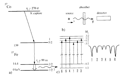
Figure 4.7. Mössbauer spectroscopy of \(^{57}\text{Fe}\). (a) The decay scheme; (b) absorption spectrometry; (c) the magnetic hyperfine spectrum.
Table 4.3. Radioactive sources for Mössbauer spectroscopy.
| Isotope | Source | \(t_{1/2}\) | \(E_{\gamma}\) (keV) | \(t_{1/2}\) (ns) |
|---|---|---|---|---|
| \(^{57}\text{Fe}\) | \(^{57}\text{Co}\) | 270 d | 14.4 | 99 |
| \(^{61}\text{Ni}\) | \(^{61}\text{Co}\) | 99 m | 67.4 | 5 |
| \(^{149}\text{Sm}\) | \(^{149}\text{Eu}\) | 106 d | 22.5 | 8 |
| \(^{155}\text{Gd}\) | \(^{155}\text{Eu}\) | 1.81 y | 86.5 | 6 |
| \(^{161}\text{Dy}\) | \(^{161}\text{Tb}\) | 6.9 d | 25.7 | 29 |
A certain fraction
\(f_{\text{M}}=\exp(-K^{2}\langle x^{2}\rangle)\) (4.7)
of decays are zero - phonon events where \(\gamma\) - rays are emitted without recoil; here \(\langle x^{2}\rangle\) is the mean - square thermal displacement of the nucleus. A similar 'Debye - Waller' factor governs the intensity of elastic x - ray and neutron scattering. The Mössbauer 'effect' is simply that these zero - phonon events have some finite probability.
Only \(\Delta M_{I}=0,\pm1\) transitions are allowed by the selection rule for dipole radiation and the relative intensities are governed by Clebsch - Gordan coefficients which depend on the angle between \(\boldsymbol{K}_{\gamma}\) and the nuclear quantization
Table 4.4. Relative intensities of Mössbauer absorption lines for \(^{57}\text{Fe}\). \(\theta\) is the angle between \(\boldsymbol{K}_{\gamma}\) and \(\boldsymbol{B}_{\text{hf}}\).
| Lines | Relative intensity | Powder average | \(\boldsymbol{B}_{\text{hf}}\parallel\boldsymbol{K}_{\gamma}\) | \(\boldsymbol{B}_{\text{hf}}\perp\boldsymbol{K}_{\gamma}\) |
|---|---|---|---|---|
| \(1,6\ (\pm3/2\rightarrow\pm1/2)\) | \(3(1 + \cos^{2}\theta)\) | 3 | 3 | 3 |
| \(2,5\ (\pm1/2\rightarrow\pm1/2)\) | \(4\sin^{2}\theta\) | 2 | 0 | 4 |
| \(3,4\ (\pm1/2\rightarrow\mp1/2)\) | \(1+\cos^{2}\theta\) | 1 | 1 | 1 |
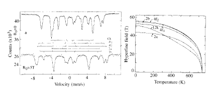
igure 4.8. The Mössbauer spectrum of \(\text{BaFe}_{12}\text{O}_{19}\). Each of the five iron sites gives rise to a six - line hyperfine pattern. An applied magnetic field allows the ferromagnetic sublattices to be resolved (Coey et al 1972).
axis. In the case of \(^{57}\text{Fe}\), there are six allowed transitions between Zeeman - split nuclear levels (figure 4.7(c)) and the \(\Delta M_{I}=0\) transitions are lines 2 and 5. The relative intensities are listed in table 4.4. For example, when \(\boldsymbol{K}_{\gamma}\parallel\boldsymbol{B}_{\text{hf}}\) the intensity of lines 2 and 5 is zero. Mössbauer spectroscopy is quite useful for determining the magnetization direction in single crystals or magnetically textured samples of iron compounds. Different crystallographic sites may be distinguished by their hyperfine spectra. The example of \(\text{BaFe}_{12}\text{O}_{19}\) is shown in figure 4.8.
Electronic Structure: Understanding the Role of Electrons in Magnetise
The dispersion relations \(E(\boldsymbol{k})\) for spin - polarized electrons are a complete description of the electronic structure of a solid. Photoemission spectroscopy gives partial information about the dispersion relations and the electronic density of states \(D(E)\). The degree of spin polarization of electrons may be inferred from spin - polarized photoemission or from tunneling or ballistic
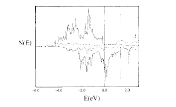
Figure 4.9. Partial densities of states for \(\text{SmCo}_{5}\). The full curves are the 3d spin density averaged over the two Co sites and the dashed curve is the 3d spin density of Sm (after Richter 1998).
point contact experiments involving a ferromagnet and a superconductor. The results are surprising insofar as electrons from iron, cobalt and nickel all exhibit a positive spin polarization of about 40%. Whereas, the measured value for the half - metallic ferromagnet \(\text{CrO}_{2}\) is 90% (Soulen 1998). Strong ferromagnets cobalt and nickel might be expected to show a negative polarization on account of the 3d\(\downarrow\) band at \(E_{\text{F}}\) but the positive polarization suggests that the electrons emitted from the 3d metals may have predominant 4s character.
The main technique for exploring the electronic structure of ferromagnets (section 2.4.2) is now computational. Density functional theory is the basis for many kinds of band - structure calculation. The electron density \(n_{\sigma}(\boldsymbol{r})\) is calculated for the ground state by numerical solution of a system of integro - differential equations involving the kinetic and potential energy of the electrons and their mutual Coulomb interaction.
The local spin density approximation (LSDA) has proved to be reliable for calculating the zero - temperature spin - polarized density of states for 3d metals and 4f - 3d intermetallic compounds (Richter 1998). By introducing spin - orbit coupling it is possible to take into account the orbital moments and estimate the 3d band anisotropy, although the anisotropic energy is only a very small fraction of the band energy. The LSDA method can also be used to calculate hyperfine interactions and crystal - field parameters. Moments of atoms on different sites in the structure are determined from the local densities of states. As an example, the overall spin - polarized density of states calculated for \(\text{SmCo}_{5}\) is illustrated in figure 4.9. Unpolarized, the method is unreliable for finite - temperature effects, such as the Curie temperature.
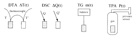
Figure 4.10. Methods of thermal analysis: the heating rate \(dT/dt\) is constant, being typically \(10\ K\ min^{-1}\).
Thermal Analysis: Examining the Temperature Dependence of Magnetic Behavior
The density of states at the Fermi level may be best deduced from the electronic specific heat. At low temperatures (typically \(1 < T < 10\ K\)) the heat capacity of a non - magnetic metal is found to vary as
\(C=\gamma_{\mathrm{e}}T+\beta_{\mathrm{ph}}T^{3}\) (4.8)
where the linear term is due to electrons and the cubic term is due to phonons. The coefficient \(\gamma_{\mathrm{e}}\) is related to the density of states of both spins at the Fermi level \(D(E_{\mathrm{F}})\), \(\gamma_{\mathrm{e}}=(1/3)\pi^{2}k_{\mathrm{B}}^{2}D(E_{\mathrm{F}})\); the linear term is normally absent in insulators. The coefficient \(\beta_{\mathrm{ph}}\) is related to the characteristic temperature \(\Theta_{\mathrm{D}}\) in the Debye model; \(\beta_{\mathrm{ph}} = 1944/\Theta_{\mathrm{D}}^{3}\). Representative values for \(\gamma_{\mathrm{e}}\) and \(\Theta_{\mathrm{D}}\) in 3d metals are \(5\ mJ\ mol^{-1}\ K^{-2}\) and \(250\ K\), respectively. Further contributions to the low - temperature specific heat arise from hyperfine interaction spin - wave excitations. In general, bosons with a dispersion relation \(\omega = Dk^{s}\) give rise to a term varying as \(T^{3/s}\). Since \(s = 2\) for isotropic ferromagnets (section 2.3.3.1), a spin - wave term proportional to \(T^{3/2}\) must be added to (4.8). The coefficient \(D_{2}\) is related to the exchange stiffness \(A\) and the exchange integrals \(J_{ij}\).
Characteristic \(\lambda\) - anomalies are observed in the heat capacity at magnetic phase transitions and there are broad Schottky anomalies associated with crystal - field excitations.
In addition to the magnetic methods discussed later in section 4.2, there is a group of thermal analysis techniques which are useful for detecting phase transitions and examining processes such as gas - solid reactions. These are differential thermal analysis (DTA), differential scanning calorimetry (DSC), thermogravimetric analysis (TGA) and thermomechanical analysis (TMA). In each case a uniform heating rate (often \(10\ C\ min^{-1}\)) is imposed and the temperature lag, heat flow, weight change or pressure change in a closed volume containing the sample is measured (figure 4.10). Thermomagnetic analysis (TMA) is a variant of TG where the sample is placed in a magnetic field gradient and the apparent weight is monitored (section 4.2.2.1).


