
Some Elementary Aspects of Magnetism: Understanding the Basics
Permanent magnets are an important part of our modern technology, and their use is increasing. The new permanent magnets based on cobalt - rare earth alloys will certainly expand the usefulness of this class of materials. It is the purpose of this chapter to present sufficient relevant introductory material to allow students, materials scientists, and engineers to become familiar with this subject. However, no attempt is made to touch on all aspects of magnetism and magnetic material, since this information can be obtained from any number of existing well - known books on these subjects (see, for example, References [1 - 6]).
Atomic Magnetism and Magnetic Alignment: Understanding the Fundamentals of Magnetization
The magnetic moment of an atom is due to the spin and orbital motions of unpaired electrons. For the ferromagnetic metals Fe, Co, and Ni, in which the unpaired electrons are the outermost ones (3d electrons), the spin contribution to the magnetic moment is the most important. The orbital angular momenta are essentially quenched. The quenching of orbital moments means that the internal electrostatic fields of the crystal reduce the orbital moment so that the moment per atom or ion is primarily due to the spin angular momentum. The lack of integral atomic moments in these metals is, according to the band model of ferromagnetism, * due to the formation, by the 3d electrons, of a narrow d band that overlaps a broad band of conduction or s electrons. The orbital motion of electrons in incomplete inner shells, such as in the rare earths, can contribute significantly to the magnetic moment of the atom.
Exchange energy or exchange forces, quantum mechanical in origin, are responsible for producing magnetic ordering in a crystal to give a net magnetic moment. Although the exchange energy is electrostatic in nature, it is sometimes convenient to think of it as a huge internal magnetic field. The elementary atomic moments should be thought of as magnetic dipoles. Exchange forces are necessary in aligning these magnetic dipoles to produce spontaneous collective atomic behavior which results in ferromagnetic, ferrimagnetic, and antiferromagnetic behavior. In Fe, Co, and Ni, the exchange interaction appears to take place via direct overlap of 3d - electron wave functions. In the case of oxides (e.g., ferrites), this
The current picture of collective behavior in these metals; see C. Herring in "Magnetism" [2].exchange interaction takes place via the nonmagnetic intervening oxygen ions and is known as superexchange. In the rare earth metals, the exchange is via polarization of conduction electrons.
Four types of magnetic behavior are schematically illustrated in Figure 1.1. It is convenient to use arrows to indicate a preferred direction of the atomic moment (also referred to as a dipole). The lengths of the arrows indicate the magnitude of the moments.
In the paramagnetic case, the exchange interactions between the atomic dipoles are so weak that the magnetic
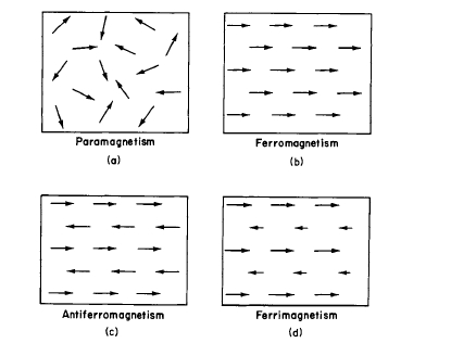
Figure 1.I Types of spin arrangement: (a) paramagnetism, no long range order of magnetic dipoles; (b) ferromagnetism, positive exchange interaction between magnetic dipoles; (c) antiferromagnetism, negative interaction between magnetic dipoles; (d) ferrimagnetism, negative interaction between unequal moments.
moments are essentially free and independent of each other. It is usually impossible to magnetize paramagnetic materials completely at room temperature (i.e., induce magnetic order) because the thermal agitation of the atoms is so great that one cannot supply sufficient magnetic field energy to overcome it.
When ferromagnetism exists, there are strong, positive exchange interactions between the atomic dipoles. The simple picture shown in Figure 1.1 indicates a parallel array of atomic moments on one magnetic sublattice. These materials are relatively easy to magnetize, and they have a high magnetic permeability.* The ferromagnetic metals Fe, Co, and Ni exhibit large moments per unit volume. If the magnitude of the atomic moment and the density of magnetic atoms are small, ferromagnets may have a small moment per unit volume. This follows from the relation \[M=\frac{mNd}{A}\] where \(M\) is the magnetic moment per cubic centimeter, \(m\) is the magnetic moment atom, \(N\) is Avogadro's number, \(d\) is the density, and \(A\) is the atomic weight.
Antiferromagnetism occurs when the exchange interaction is negative and the opposing moments are equal. In the simple picture shown in Figure 1.1, equal magnetic moments, on two sublattices, point in opposite directions. The moments on each
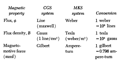
* The magnetic permeability is equal to the magnetic flux - density \(B\), in gauss, in the material divided by the magnetizing force \(H\), in oersteds. In this work we will use the CGS system of units, since most of the data in the literature are given in these units. Conversions between the CGS and MKS systems are given in Appendix 1.1.sublattice may be canted. Nevertheless, the net atomic moments of each sublattice cancel and result in a zero net moment. These materials are difficult to magnetize and have low magnetic permeability.
Ferrimagnetism occurs in solids containing more than one magnetic sublattice when the exchange interactions are negative but the oppositely directed atomic moments on each sub - lattice are unequal, resulting in a net magnetic moment. This can occur when at least two different species of magnetic atoms or ions with different moments are present in the crystal. Although Figure 1.1 illustrates an antiparallel arrangement of the direction of the atomic moments on each sublattice, the moment directions can be related by some angle from one another. These materials are relatively easy to magnetize and exhibit many of the properties of ferromagnets. Examples of commercially important ferrimagnetic materials are ferrites and garnets.
Magnetic Domains: Structure, Behavior, and Their Role in Magnetism
Although spontaneous alignment or order of the atomic moments exists in ferro - and ferri - magnets, these materials often do not show a net moment in the absence of an applied field. This is due to the existence of magnetic domains in the material. Domains are small regions within which the elementary magnetic dipoles or atomic moments are oriented by the exchange energy so that they are parallel. Figure 1.2 shows a schematic view of such domains in a section of a demagnetized bar. In this state, the net moment of the material as a whole is zero. The reason for this is that the domains are oriented in
such a way that their moments cancel so as to minimize the total magnetic energy.
The transition region between domains is called a domain wall. Domain widths frequently range between \(10^{-3}\) and \(10^{-5}\) cm. Domain wall thicknesses are of the order of 1000 atoms in an iron crystal.* The walls between domains whose moments are oriented in opposite directions are called \(180^{\circ}\) walls; domains at right angles are separated by \(90^{\circ}\) walls. A \(180^{\circ}\) domain wall is shown in Figure 1.3, which schematically illustrates how the atomic moments appear in this region.
The domain structure and the behavior of domains and domain walls in an applied magnetic field determine many of the magnetic properties in ferro - and ferrimagnetic materials. In materials that are easy to magnetize and demagnetize (known as soft magnetic materials such as iron - silicon alloys, the magnetic domains are usually large; by using the magnetic powder pattern technique† one may observe them by means of an ordinary microscope. In general, if a magnetic field is applied, a change in the domain structure will be observed. In materials that are hard to magnetize and demagnetize (known as hard magnetic materials), the domains are very small and in many cases cannot be observed in detail with an ordinary microscope. In some materials, they can be viewed under polarized light. In general, the polarized light is either reflected from the surface of the specimen as shown in Figure 1.4 (Kerr magneto - optical effect) or transmitted through thin
* In rare earth permanent magnet alloys, domain wall widths are approximately \(10^{-6}\) cm (see Chapter IV).† Instructions for making the magnetic colloid and preparing the metal surface for viewing domains are given in Appendix 1.2.
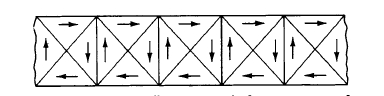
Figure 1.2 Schematic illustration of domains in a demagnetized iron bar. Each triangular area represents a magnetic domain composed of many parallel - oriented dipoles.
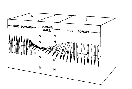
Figure 1.3 Illustration of the change in orientation of atomic moments across a 180° domain wall.
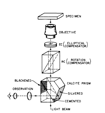
Figure 1.4 The Kerr method for observing domains. In this method, the ferromagnetic crystal is viewed by plane polarized light reflected from the surface.
films as shown in Figure 1.5 (Faraday effect). In some cases, oblique transmission is used.
Domains and their behavior have been studied extensively during the past two decades. Magnetic domains observed by Bobeck [7] in a special garnet crystal (a soft magnetic material) are shown in Figure 1.6. The small circular domains shown in the lower right of Figure 1.6 can be manipulated to perform memory and logic functions. The ability to control these domains is the basis of a new magnetic "bubble" memory. The mixed garnet and related materials, are referred to as magnetic "bubble" materials. Figure 1.7 shows magnetic domains in \(\text{Co}_{5}\text{Sm}\), which is a hard magnetic material when used in fine - particle form. The photograph was taken by using
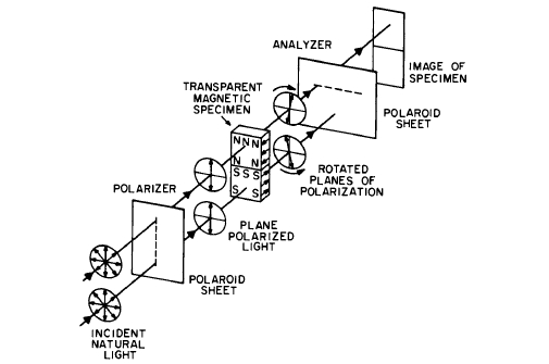
Figure 1.5 The Faraday method for observing domains by means of polarized light. Transparent materials are usually studied by this technique.
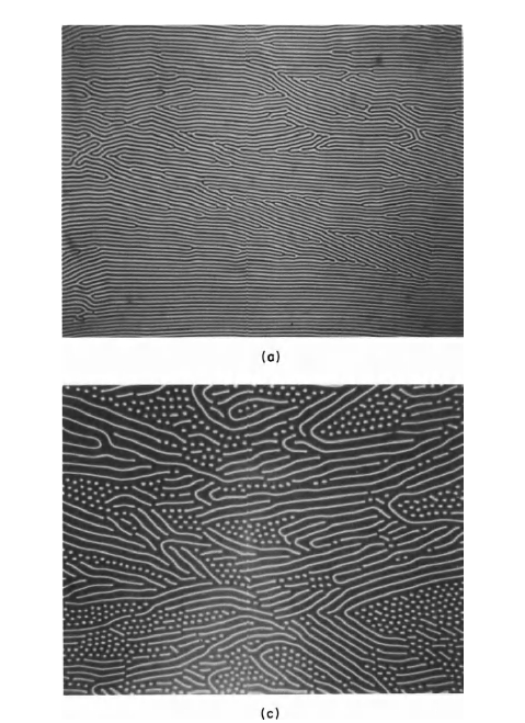
Figure 1.6 Domain patterns in a 2 mil thick, (111) platelet of \(\text{Gd}_{0.94}\text{Tb}_{0.75}\text{Er}_{0.31}\text{Al}_{0.5}\text{Fe}_{4.5}\text{O}_{12}\) garnet (a). Bias or applied field normal to the platelet surface (b). Same except strip domains have been "cut" with a magnetic wire probe to break
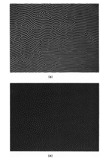
up some of the strip domains (c). In (d), bias field is 150 Oe to create cylindrical domain array. The "bubbles" or cylindrical domains are 5 \(\mu m\) in diameter (after Bobeck [7]). No cylindrical domains will be present if the applied field reaches the saturation value. Domains observed by use of the Faraday effect.
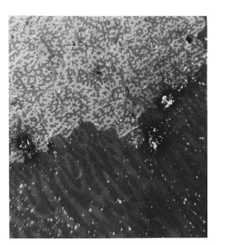
Figure 1.7 Domain pattern of \(\text{Co}_{5}\text{Sm}\), which shows domains perpendicular (upper left portion of figure) and parallel to the hexagonal axis of the crystal (lower right portion).
a polarizing microscope and utilizing the Kerr magneto - optic effect.
Magnetization: Principles, Processes, and Applications
The process of magnetizing a ferro - or ferrimagnetic material involves the movement of domain walls and rotation of the magnetization vectors of the domains. For example, if one magnetizes a thin rod of iron, a magnetization of \(4\pi M\) gauss is established, which is due to the movement and reorientation of the magnetization vectors of the magnetic domains. In addition, the magnetizing field of \(H\) oersteds is also present in the volume occupied by the iron. The sum of these terms, \(4\pi M + H\), is called the magnetic flux density \(B\). Hence, the basic equation is \[B = 4\pi M+H\] where \(B\) is measured in gauss. Figure 1.8 illustrates schematically how the domain structure of a magnetic material changes as it is magnetized to saturation. Initially there are four triangular domains (sample demagnetized, zero net magnetic moment), which finally become a single domain oriented in the direction of the applied field. Note that domain wall motion is the mechanism for the magnetization process in low applied fields, whereas rotation of the atomic moments is the mechanism for high applied fields.
Magnetic hysteresis is an important characteristic property of ferro - and ferrimagnetic materials; it is not exhibited by paramagnetic substances. Figure 1.9 shows a magnetization curve and hysteresis loop of iron. These curves enable us to define various terms used in magnetism to characterize the
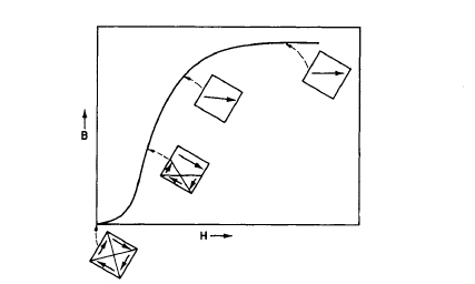
Figure 1.8 Schematic illustration of domain structure at various stages of the magnetization process.
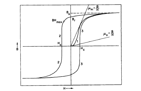
Figure 1.9 Ferromagnetic magnetization curve and hysteresis loop. Important magnetic quantities are illustrated.
magnetic properties of a material. On the application of a magnetic field \(H\), a net magnetization is established, and upon plotting the value of \(B\) as a function of \(H\), curve 1 is obtained. The maximum value of \(B\) reached is referred to as \(B_s\). If the applied field is reduced to zero, the value of \(B\) does not return to zero but traces curve 2 to the point \(B_r\). If the \(H\) field is now reversed in direction and increased in a negative direction, the curve continues along 2 until \(B\) equals \(-B_s\). If \(H\) is again decreased to zero and then reversed in direction, curve 3 will be obtained and the hysteresis loop will be completed. The mechanism of magnetic hysteresis can be understood from the magnetic powder pattern photograph of a silicon - iron crystal shown in Figure 1.10. The presence of small imperfections has an important effect on the hysteresis or demagnetization be - havior of magnetic materials. The reason for this is that an imperfection impedes domain wall motion and spikelike do - mains develop, lowering the total magnetic energy. In Figure 1.10, when the domain boundaries pass through an imperfec - tion, these spikelike domains cling to it, stretch, and finally snap off. Imperfections in a material, such as solute impurities, dislocations, grain boundaries, and other phases, are an im - portant source of magnetic hysteresis.
The area enclosed by the hysteresis loop is a measure of the hysteresis loss, the latter being designated \(W_h\). The quantity \(B_s\) is known as the saturation induction and \(B_r\) as the residual induction that remains when the applied field is reduced to zero. \(H_c\) is the coercive force; it is the reverse field required to reduce \(B\) to zero. For permanent magnets, it is important that this term be large enough to resist external demagnetizing forces that tend to reduce the flux to zero. Sometimes the intrinsic coercive force, \(_iH_c\) or \(H_{ci}\), is used; it is the field necessary to reduce \((B - H)\) to zero. When this is done, the quantity \((B - H)\) is plotted instead of \(B\)
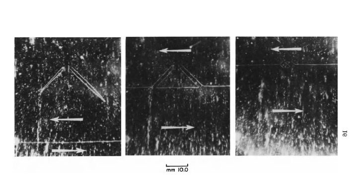
Figure 1.10 Magnetic powder pattern photograph of a domain structure in silicon - iron that shows a 180° domain boundary moving through an imperfection under the influence of an applied magnetic field. As the boundary moves through the imperfection, the spike - like domains cling to the boundary, stretch, and finally snap off. The impeding of domain wall motion by imperfections is an important source of magnetic hysteresis.
on the ordinate. For rare earth permanent magnets, \(_mH_c\) is usually much greater than \(H_c\). For the Alnico type magnets, in which \(B\) is usually much larger than \(H\), the values of \(H_c\) and \(_mH_c\) are quite comparable. The value \((BH)_{max}\) indicated in the second quadrant (Figure 1.9) is known as the maximum energy product and is a figure of merit for permanent magnet materials. This point represents the optimum condition, in which a given amount of flux will be carried by the smallest amount of material. For some permanent magnet applications, where demagnetizing forces are large and variable, the magnitude of intrinsic coercive force is of great importance. \((BH)_{max}\) enters into equations used in the design of permanent magnets (Appendix 1.3).
The initial permeability \(\mu_{0}\) is determined by the initial slope of the magnetization curve, and the maximum permeability \(\mu_{m}\) is determined by the maximum ratio of \(B/H\) of the magnetization curve, as illustrated in Figure 1.9. Another term closely related to the permeability is the susceptibility \(k\), which is equal to the ratio \(M/H\), where \(M\) is the magnetization. Usually the susceptibility is expressed in electromagnetic units (emu) per gram and is then designated \(\chi\), which is equal to the ratio \(\sigma_{g}/H\), where \(\sigma_{g}\) is the magnetic moment per gram.
Thermal Variation of Magnetization: How Temperature Affects Magnetic Properties
Curves of magnetization versus temperature yield fundamental information on the nature of the coupling between atomic dipoles. The thermal variation of the magnetization for iron is shown in Figure 1.11. The shape of this curve is typical for ferromagnetic materials. Increasing the temperature
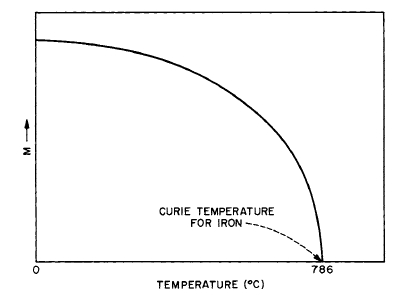
Figure 1.11 Variation of intrinsic magnetization \(M\) with temperature for iron. At \(786^{\circ}C\), the magnetization becomes practically zero; the temperature at which this occurs is known as the Curie temperature.
results in disordering of the long - range magnetic order. At \(786^{\circ}C\), the long - range alignment of the atomic dipoles due to exchange energy is completely destroyed. This temperature is known as the Curie temperature (\(T_C\)); above it, iron is paramagnetic. At the Curie point the magnitude of the thermal energy of the atoms is of the order of the energy corresponding to the exchange field. On this basis, the value of the exchange field turns out to be of the order of \(10^7\) Oe. This field is more intense than can be produced in the laboratory.
The variation of magnetization with temperature for ferrimagnetic materials is usually more complicated. Six possible types of temperature dependency are illustrated in Figure 1.12 [8], and they have been observed experimentally. The
most interesting aspect of these curves is the appearance of a compensation temperature \(\theta_{K}\), as shown in Figures 1.12d and 1.12f. At the temperature \(\theta_{K}\), the magnetizations of two sublattices are equal and opposite and the resultant magnetization is zero. When the temperature rises above \(\theta_{K}\), the magnetizations of the two sublattices are no longer equal and the resultant magnetization increases to a maximum and finally disappears at the Curie point \(\theta\).
Antiferromagnetic coupling is frequently detected by plotting the susceptibility against temperature as shown in Figure 1.13 for \(\text{NiMoO}_{4}\). This material becomes antiferromagnetic at approximately \(19^{\circ}\text{K}\), which is indicated by the sharp peak
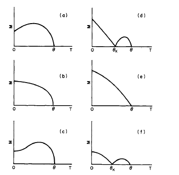
Figure 1.12 (a) - (f) Examples illustrating the manner in which the magnetization may vary in ferrimagnetic materials. \(\theta\) is the Curie point and \(\theta_{K}\) is the point of compensation.
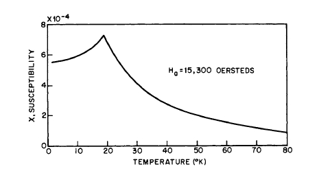
Figure 1.13 Susceptibility of \(\text{NiMoO}_{4}\) with temperature (L. G. Van Uitert, R. C. Sherwood, H. J. Williams, J. J. Rubin, and W. A. Bonner). The temperature at which the maximum in susceptibility occurs is approximately the Néel point.
(Néel point) in the susceptibility curve. Above \(19^{\circ}\text{K}\) the material is paramagnetic.
Magnetic Anisotropy: Directional Dependence and Its Impact on Materials
High magnetic anisotropies are important in determining the properties of permanent magnet materials. For example, in fine - particle magnets such as Alnico, reversals in magnetization are opposed by high anisotropic forces. This results in the material having a high coercive force. The rare earth permanent magnets have the highest coercive forces and also the highest values of magnetic anisotropy. Anisotropies can be classified as magnetocrystalline, shape, strain, and pair ordering (or deformation - induced for ductile magnetic alloys).
a. Magnetocrystalline anisotropy is the result of the exist -
ence of preferred crystalline axes for magnetization (the preferred directions for the magnetic dipoles); it is an intrinsic property of the material. The energy required to rotate the magnetization vector from the easy to the hard direction of magnetization is a measure of the magnetocrystalline anisotropy. Some permanent - magnet materials that depend on this type of magnetic anisotropy for their magnetic behavior are intermetallic compounds of cobalt and rare earths, \(\text{MnBi}\), and barium and strontium ferrites. If the crystal anisotropy \(K\) is known, one can calculate the theoretical maximum coercive force of a small particle for which magnetocrystalline anisotropy dominates and coherent domain rotation (all the domain vectors rotate in unison) is the only magnetic process [9]. The equation for performing this calculation is \[H_{c}=\frac{2K}{M_{s}}\] where \(M_{s}\) is the saturation magnetization. \(H_{c}\), determined from this equation, is also referred to as the anisotropy field \(H_{A}\). \(H_{A}\), and thus \(K\), can be estimated by determining the magnetization behavior in the easy and hard directions (Figure 1.14) on single crystals or sometimes on magnetically aligned powders frozen in wax. The anisotropy field is estimated by extrapolating the hard - axis curve to saturation. Thus, the anisotropy field is the field required to rotate the magnetization into the hard direction or the field required to saturate the material in the hard direction, and it is a measure of the anisotropy.
As indicated, the above equation holds for a magnetization process that involves only coherent domain rotation; however, when small particles contain imperfections or surface irregularities (which is usually the case), the reversal of the magnetization may not occur coherently and the coercive force will be less than that calculated from the above equa -
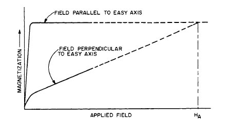
Figure 1.14 Schematic illustration of magnetization curves obtained when the applied field is parallel and perpendicular to the easy axis of magnetization. Data of this sort on single crystals or on previously aligned powders frozen in wax allow for an estimate of the anisotropy field by extrapolating the hard - axis magnetization to saturation. Thus, the anisotropy field is the field required to rotate the magnetization into the hard direction and is a measure of the anisotropy of the material. In many cases, a reverse domain is nucleated and the magnetization reverses by domain wall movement.
b. Shape anisotropy is the preferential alignment of atomic moments in a given direction due to the shape of the magnetic particle. In Alnico, the precipitate is magnetic and has shape anisotropy that accounts for the coercive force of the alloy. For an elongated small particle, it is easy to magnetize parallel to the long dimension (small demagnetizing factor*).
* An elongated particle or rod, when magnetized, creates a demagnetizing field itself, which is in opposition to the applied field. It is approximately proportional to the intensity of magnetization \(M\) and the demagnetizing factor \(N\). The latter depends on the ratio of length/diameter of the elongated particle or rod. These values may be found in Bozorth [1].and difficult to magnetize normal to it (large demagnetizing factor), and the magnetization vector will lie along the length of the particle. The ratio of the length to the width of the particle is a measure of its shape anisotropy. Since high shape anisotropy results in good permanent magnet proper - ties in small particles, needle - like shapes are very desirable for this type of anisotropy to be effective. The coercive force of an elongated particles for which shape anisotropy is dominant may be calculated [9] from the equation \[H_{c}=(N_{t}-N_{0})M_{s}\] where \(N_{t}\) is the demagnetizing factor in the narrow direction and \(N_{0}\) is the demagnetizing factor in the long direction.
c. Strain or magnetostriction anisotropy, as the name im - plies, is produced by a combination of strain and magnetostriction in the crystal. The application of a stress along a given crystallographic direction may result in an increase or decrease in the magnetization for a given applied field along that direction. Strain sensitivity is denoted in terms of magnetostriction constants and is a measure of the change in length of a sample in the direction of the applied field. Magnetostriction constants can be positive, zero, or negative. A positive magnetostrictive constant for a given crystal direc - tion means that strain in this direction will aid magnetizing along this direction. Conversely, the material will elongate in this direction in an applied field. If tension is applied to a magnetic material having positive magnetostriction, the domains will line up along the axis of tension. Energy will be required to rotate the domains out of this easy direction, and therefore a uniaxial anisotropy has been established. The general importance of this phenomenon for many commer - cial permanent magnet applications is not known. However, the coercive force of the ductile age - hardened iron - cobalt -
vanadium alloys (Vicalloys), which are quite magnetostrictive, show a strong dependence on applied stress. Stoner and Wohlfarth [10] give the following equation relating the coercive force to the uniaxial stress \(T\) and magnetostriction constant \(\lambda\): \[H_{c}=\frac{3\lambda T}{M_{s}}\]
d. Pair ordering [5] results in a uniaxial anisotropy due to an asymmetrical distribution of like or unlike atom pairs in an alloy or compound. This distribution can be induced as a result of heat treatment in a magnetic field or plastic deformation, as in Fe - Ni alloys (Permalloys).
Permanent Magnet Materials: Properties, Types, and Technological Applicationss
It is an experimental fact that for certain ranges of particle size, the intrinsic coercive force of a ferromagnetic material increases as the particle size decreases. For iron it reaches a maximum at approximately a diameter of 100 Å, and for the compound MnBi it increases from 1000 Oe at 70 μm to 12,000 Oe at 5 μm. Eventually, as the particle size is further reduced, the coercive force decreases because of the occurrence of superparamagnetism* or other causes, such as the presence of a large concentration of crystalline defects and structural changes. The rodlike precipitates in Alnico, which are responsible for the coercive force of this alloy,
* Superparamagnetism occurs when the particles become so small that their direction of easy magnetization is no longer stable because of thermal agitation. In iron this occurs in the vicinity of 30 – 40 Å diameter particles.
have a diameter of approximately 200 Å. When the Alnico particles are larger than 200 Å in diameter, the coercive force of the alloy is much lower. For example, at 1000 Å the coercive force would be of the order of 20 Oe. The fine – particle theory of coercive force predicts such behavior. This theory simply states that when the particle becomes so small that it is energetically unfavorable for domain walls to exist, there will be only one domain present in the particle and the magnetization change will take place by a rotation mechanism. The theory is thought to apply to the Alnicos, but does not apply to the cobalt – rare earth magnets prepared by powder metallurgy techniques (Chapter V). For this class of materials, substantial evidence exists that indicates that the coercive force is still determined by nucleation and growth of reverse domains and by the pinning of domain walls [11, 12], even in particles as small as 10 μm.</p>
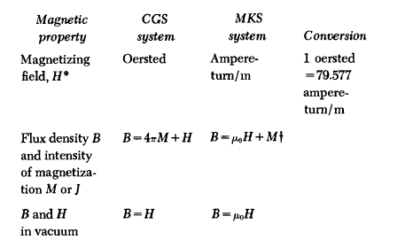
Appendix 1.1
Appendix 1.2
Instructions for Making a Colloidal Suspension of Magnetite and Preparing Metal Surfaces for Microscopic Observation of Domains
To obtain a suitable sample of magnetite (\(\text{Fe}_{3}\text{O}_{4}\)), 2 g of ferrous chloride (\(\text{FeCl}_{2}\cdot4\text{H}_{2}\text{O}\)) and 5.4 g of ferric chloride (\(\text{FeCl}_{3}\cdot6\text{H}_{2}\text{O}\)) are dissolved in 300 ml of hot water. A solution consisting of 5 g of sodium hydroxide in 50 ml of water is then added, while constantly stirring, to the first solution. When the sodium hydroxide solution is added, a black precipitate will form. The precipitate is allowed to settle to the bottom of the beaker; this will take about five minutes.
* Terrestrial magnetic fields are measured in units of gammas, where 1 gamma \( = 10^{-5}\) gauss \(=10^{-9}\) tesla.
† In the MKS system \(\mu_{0}=4\pi\times 10^{-7}\)
clear liquid, which contains excess salt and caustic, is then carefully removed and the residue transferred to a 2000 - ml beaker or its equivalent which is filled with distilled water and stirred. The precipitate is allowed to settle again and the clear liquid removed. The purpose of this procedure is to thoroughly wash the precipitate. The precipitate should be washed in this manner twice more. As the precipitate becomes cleaner, it takes progressively longer to settle (approximately two hours). About one inch of liquid and precipitate should be in the beaker after following the above recipe.
The precipitate is then stabilized by adding a solution prepared as follows:
- Place 5 g of dodecyl amine acetate (Armac C from Armour & Co.) in a 1000 ml beaker.
- Next add about 300 ml of water and gently warm the beaker to melt the acetate.
The stabilizing solution is then combined with the precipitate and must be thoroughly mixed. This is an important part of the procedure. This can be accomplished easily by placing about 150 ml of the mixture in a high - speed food blender and stirring for about 10 min. The colloid is now ready for use.
The proper preparation of metallic surfaces is very important, and has been a major factor in the history of investigation of magnetic domains. When the surface of a metal is properly prepared for magnetic domain examination, the surface should not have any obvious ridges or saw marks. If these are present, they should be removed with 400 - mesh or coarser abrasive paper. The surface should then be hand - lapped with 600 - mesh paper and finished with 00 French emery. The final and most important step is to remove the strained material from the surface by electropolishing. The electropolishing equipment consists of a 300 - ml beaker con -
taining ¼ lb of chromic trioxide \(\text{CrO}_{3}\) and 1 pt of phosphoric acid. This is a standard electropolishing solution. The specimen is grasped by a combination of tweezers and battery clip. The specimen serves as the anode and a copper electrode as a cathode with an applied voltage of 18 V. Usually 5 - 10 min of operation is sufficient to remove strained material from a surface that has had light mechanical polishing.
The specimen should be examined at 1 - to 2 - min intervals to check the progress of the polishing, and should finally appear to have a mirrorlike surface. Under the microscope without colloid, the specimen should appear smooth and dark. After the specimen is viewed the colloid should be washed off by holding it under a stream of water, rubbed lightly with tissue, and then dried by blowing air across its surface.
Appendix 1.3
Equations Used for Design of Permanent Magnets
The basic design equations are \[FH_{g}A_{g}=B_{d}A_{m}\quad(1)\] \[fH_{g}l_{g}=H_{d}l_{m}\quad(2)\] where \(F\) is the leakage coefficient, which is the ratio of the total flux in the magnet to the useful flux in the air gap. \(H_{g}=\) magnetizing force or flux density in the air gap. \(A_{g}=\) cross - sectional area of the air gap at right angles to the lines of flux.
\(B_{d}=\) flux density in magnet at operating point on demagnetization curve.
\(A_{m}=\) area of magnet at right angles to the direction of magnetization.
\(f =\) reluctance factor, which takes account of the fact that the flux in the air gap is not everywhere perpendicular to the pole face and therefore the length of path is greater than the geometrical value \(l_{g}\). Also it accounts for the mmf drop in the soft iron and joints.
\(l_{g}=\) length of air gap.
\(H_{d}=\) the field in the magnet at the operating point on the demagnetization curve.
\(l_{m}=\) length of magnet.
By multiplying (1) and (2), \(FfH_{g}^{2}A_{g}l_{g}=B_{d}H_{d}A_{m}l_{m}\) and \(\text{Volume}_{gap}=A_{g}l_{g}\). Then \[V_{m}=\frac{FfH_{g}^{2}V_{g}}{B_{d}H_{d}}\quad(3)\] Equation (3) shows that the volume of the magnet is inversely proportional to the energy product and that the volume of the magnet is a minimum when \(B_{d}H_{d}\) is a maximum.
In addition, by dividing (1) by (2), \[\frac{B_{d}}{H_{d}}=\frac{FA_{g}l_{m}}{fl_{g}A_{m}}\quad(4)\] The ratio \(B_{d}/H_{d}\) is known as the permeance coefficient. Equation (4) states that this ratio is determined by the area \(A_{m}\) and length \(l_{m}\) of the magnet, the area \(A_{g}\) and length \(l_{g}\) of the air gap, and the leakage \(F\) and reluctance \(f\) factors. The terms \(F\) and \(f\) vary in different magnetic structures and usually cannot be calculated accurately. Permanent - magnet designers can usually estimate their values from previous experience.
The reluctance factor \(f\) usually varies from 1.0 to 1.5. The leakage factor \(F\) can be estimated as follows: \[F=\frac{P_{t}}{P_{g}}\] where \(P_{t}\) is the total permeance and \(P_{g}\) is the gap permeance \(A_{g}/L_{g}\). The total permeance can be obtained by breaking up the field into probable flux paths that have simple geometric shapes which are amenable to calculation. Then \[F=\frac{P_{t}}{P_{g}}=\frac{P_{g}+P_{1}+P_{2}+\cdots+P_{n}}{P_{g}}\]
Further information can be obtained on this method and others from Parker and Studder [13], Roters [14], and Had - field [15].


