

6.3 Dynamic Applications with Mechanical Recoil: Harnessing Magnetic Motion
Permanent - magnet structures can be adapted to produce a variable field by some change of the air - gap or movement of the magnets with respect to one another. The working point is displaced as the magnets move, or turn, so these devices involve mechanical recoil.
Variable Flux Sources: Controlling Magnetic Fields for Efficiencys
To create a uniform variable field, two Halbach cylinders of the type shown in figure 6.7(d) with the same radius ratio \(\rho=r_{2}/r_{1}\) can be nested inside each other. Then by rotating them through an angle \(\pm\alpha\) about their common axis, a variable field \(2B_{\text{r}}\rho\cos\alpha\) is generated. A practical realization of such a device is shown in figure 6.15(a). Another solution is to rotate the rods in the device of figure 6.7(e). By gearing a mangle with an even number of rods
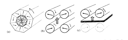
Figure 6.15. Permanent-magnet variable flux sources: (a ) a double Halbach cylinder , (b ) a four- rod mangle and (c ) a two-rod mangle with a magnetic mirror.
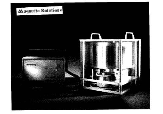
Figure 6.16. A permanent - magnet variable flux source and controller. The magnet head, based on the design of figure 6.15(a), produces a variable field of up to 1.8 T in any transverse direction in the bore. (Courtesy of D Hurley, Magnetic Solutions Ltd.)
so that the alternate rods rotate clockwise and anticlockwise though an angle \(\alpha\), the field varies as \(B_{\text{max}}\cos\alpha\). Further simplification is possible with a magnetic mirror (figure 6.9). The number of rods needed in a mangle may be halved by using a sheet of soft iron, as shown in figure 6.15(c). A field gradient which moves along the axis can be obtained by rotating the rods of a mangle which are magnetized so that their direction of magnetization twists along their length (section 6.2.2).
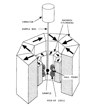
Figure 6.17. A schematic of a vector vibrating - sample magnetometer using a permanent - magnet flux source of the type shown in figure 6.16 (Ingram 1994).
These permanent - magnet variable flux sources are compact and particularly convenient to use since they can be driven by stepping motors or servomotors and they have none of the high power and cooling requirements of a comparable electromagnet. For example, a variable - field source giving a maximum field of Nd - Fe - B magnet of the design shown in figure 6.15(a) to generate 3.8 T is a 25 mm bore. These devices are very convenient for compact magnetic measurement systems such as the Vector Vibrating - sample Magnetometer illustrated in figure 6.17.
Large alternating fields can be generated by rotating the magnets relative to one another. Peak fields of 1.5 T and mean fields of up to 1 T at a frequency of several hertz, with access along three axes, are available in a variable - field system of this type.
The limit to the fields that can be continuously generated using permanent magnets is set in part by the coercivity and anisotropy field of the material since demagnetization will occur if the field exceeds these values. Nevertheless, the field in the bore. However, there is also the practical size limitation imposed by (6.3). Admitting that material exists with \(B_{\text{r}} = 1.5\ T,\mu_{0}H_{\text{c}} = 5\ T\) and
\(\mu_{0}H_{\text{c}}>10\ T\), the diameter of the cylinder required to achieve 5 T in a 25 mm bore would be 700 mm. Such a structure 400 mm high would weigh about a tonne. A pulsed - field magnet can be used to generate much higher fields to displace hysteresisloops to greater fields of up to about 2 T, but they cannot compete with superconducting solenoids in the higher field range.
Switchable Magnets and Holding Magnets: Versatile Magnetic Solutions
A simple type of variable flux source is the switchable magnet. In one version, the field is changed from \(\pm B_{\text{r}}\) to zero by rotating a permanent magnet structure relative to a fixed set of soft - iron pole - pieces. More common are magnetic holding devices, where a strong force is exerted on a piece of ferrous metal in contact with the magnet. The working point shifts from the knee of the \(B - H\) loop to a point close to the remanence when the circuit is closed. The maximum force \(F\) that can be exerted at the face of a magnet of area \(A\) and flux density \(B\) is given by \(F = B^{2}A/2\mu_{0}\). For a C - shaped segment which are then separated by a small distance \(d\), the energy appearing in the air - gap is \(2\times(1/2\mu_{0})B_{\text{r}}^{2}A_{\text{g}}d = B_{\text{r}}^{2}A_{\text{g}}d/\mu_{0}\). The work done separating the segments is \(Fd\), hence the force per unit area is \[F/A=\frac{B_{\text{r}}^{2}}{2\mu_{0}}\] (6.13) Forces of up to \(40\ N\ cm^{-2}\) can be achieved for \(B_{\text{r}} = 1\ T\).
Large quantities of isotropic sintered ferrite are used for catches and闩锁in domestic appliances and for freezer - holding magnets. Isotropic plastic - bonded ferrite with \(B_{\text{r}}\approx0.1\ T\) is used for magnetic notice boards and probably a few millinewtons wide. It attaches itself to any mild - steel surface such as a refrigerator door. A typical holding force is \(0.1\ N\) for a \(100\ cm^{2}\) area. There are many other uses of holding magnets. For example, small rare - earth magnets used in latches are used to hold doors.
Another form of switchable magnet is illustrated in figure 6.19. By means of a lever, the permanent magnet is rotated or displaced from an 'off' position, where the return path is provided by the soft - iron in the device, to an 'on' position where the magnetic circuit is completed through a steel hook to which the clamp is firmly attached.
Magnetic Couplings and Bearings: Enhancing Motion and Durabilitys
Permanent magnets are useful for coupling rotary or linear motion when no contact between members is allowed (Yerman 1990), for example across the wall of a vacuum or pressurized volume or in an aggressive chemical environment. Figure 6.20 illustrates a simple arrangement for coupling the motion of two gears. Forces depend quadratically on the remanence of the magnets, so it is advantageous to select material with a large magnetization. If the coupling
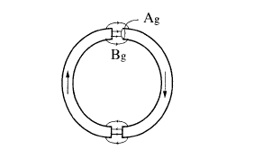
Figure 6.18. A magnetic toroid, cut and separated to produce a field in the airgap.
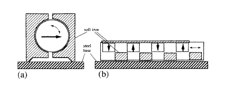
Figure 6.19. Two designs for switchable magnetic clamps. (a) is a rotatable magnet design, shown in the 'on' position, and (b) is a design where the magnet array is displaced laterally, shown in the 'off' position.
slips, the magnets may be subjected to a substantial reverse field, so a high coercivity is also required. Rare - earth magnets are ideal for these applications. The torque varies sinusoidally with the relative angular displacement of the two members of the coupling with period \(4\pi/p\), where \(p\) is the number of poles in each. The maximum torque can be varied by adjusting the air - gap. Torques of order 10 N m may be achieved in couplings a few centimetres in dimension.
Magnetic bearings are simple, cheap and reliable. They are well - suited to high - speed rotary suspensions in flywheels or turbopumps, for example. Linear suspensions have been tested in prototype magnetically levitated transportation systems. It is a feature of magnetic bearings that a mechanical constraint (or active electromagnetic support) is generally required in one direction. The simplest bearings are made of two ring - shaped magnets in repulsion. Figure 6.21(a) shows a configuration which provides a radial restoring force provided the axis is prevented from shifting or twisting. The configuration in figure 6.21(b) supports a load in the axial direction, but it must be prevented from moving in the radial direction.
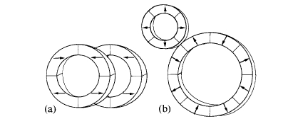
Figure 6.20. (a ) A face-type coupling with four axially magnetized segments , (b) A 2:1 magnetic gear with radially magnetized segments

Figure 6.21. Two elementary magnetic bearings made from axially magnetized rings; (a) a radial bearing and (b) an axial bearing.
If the axial and radial components of the forces on these bearings are \(F_{z}\) and \(F_{r}\), the corresponding diagonal stiffnesses \(K_{z}\) and \(K_{r}\) are defined as \(-\text{d}F_{z}/\text{d}z\) and \(-\text{d}F_{r}/\text{d}r\), respectively. When \(K_{i}\) is positive, \(F_{i}\) is a restoring force and the bearing is stable in that direction. In absolute stable equilibrium, \(F_{i} = 0\) and \(K_{i}>0\) for all components. Sadly, this cannot be achieved solely by static magnetic forces acting on a permanent magnet. It follows from Maxwell's equation \(\nabla\cdot\boldsymbol{B}=0\) that \(\nabla\cdot\boldsymbol{F}=\nabla^{2}(\boldsymbol{m}\cdot\boldsymbol{B}_{0}) = 0\), where the force \(\boldsymbol{F}\) on a magnet of moment \(\boldsymbol{m}\) is \(\nabla(\boldsymbol{m}\cdot\boldsymbol{B}_{0})\). Hence, \[K_{x}+K_{y}+K_{z}=0\] (6.14) It is therefore impossible to achieve stability in all three directions, a result known as Earnshaw's theorem. For a cylindrical bearing, \(2K_{r}+K_{z}=0\); hence if \(K_{z}\) is positive, \(K_{r}\) is negative and the axial bearing is unstable along the axis. Conversely, if \(K_{r}\) is positive, \(K_{z}\) is negative and the radial bearing is unstable along the axis.
The linear magnetic bearing shown in figure 6.22 provides levitation along a track, but lateral constraint is required. It is impracticable to equip a great length of track with permanent magnets, so instead levitation may be provided by repulsion from eddy currents generated in a track of aluminium plates by permanent magnets attached to the base of the moving vehicle (figure 6.23) or by attraction of the magnets on the vehicle to a suspended iron rail.
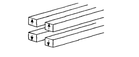
Figure 6.22. A linear magnetic bearing.
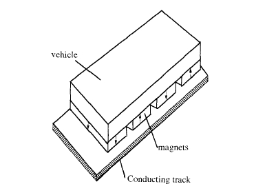
Figure 6.23. A Maglev system where the suspension depends on eddy-current repulsion.
To calculate forces produced in magnetic bearings and couplings made up of uniformly magnetized blocks or ring - shaped magnets with rigid magnetization, it is convenient to use the surface charge method (Yonnet 1996), which was introduced in section 2.1.1.2. A uniformly magnetized block with magnetization \(\boldsymbol{e}_{n}M\) is magnetically equivalent to sheets of surface charge \(\sigma_{m}=\mu_{0}\boldsymbol{M}\cdot\boldsymbol{e}_{n}\), where \(\boldsymbol{e}_{n}\) is the surface normal. The radial field \(H\) due to a small charge \(\sigma_{m}\text{d}S\) is \(\sigma_{m}\text{d}S/4\pi r^{2}\) and the force on a charge \(\sigma_{m}\text{d}S\) in a field \(\boldsymbol{H}\) is \(\mu_{0}\boldsymbol{H}\sigma_{m}\text{d}S\).
The magnetic hinge is a special type of magnetic bearing designed to compensate gravitational torque on an arm. It is illustrated in figure 6.24. The torque on the arm is \(\Gamma = m'gl\sin\alpha\), where \(m'\) is the suspended mass, which may be compensated at any angular position \(\alpha\) by the torque \(m\boldsymbol{B}\sin\alpha\) on a magnet of moment \(m\) in the axial turn in a region of uniform field \(\boldsymbol{B}\) produced by a magic cylinder magnet of the type discussed in section 6.2.1.
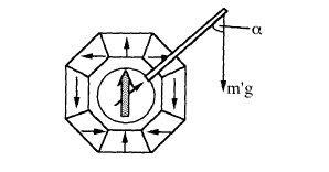
Figure 6.24. A magnetically compensated hinge.
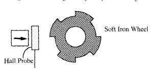
Figure 6.25. A variable-reluctance sensor.
Magnetic Sensors: Precision Detection and Measurement
Magnetic sensors are based on detecting a varying field in an air - gap using a Hall effect or magnetoresistance probe which delivers a voltage depending on \(B\). Magnetic position and speed sensors are used in brushless motors and automobile system controls, where they offer reliable non - contact sensing in a hostile environment involving dirt, vibration and high temperatures. Examples are crankshaft position sensors, sensors for anti - lock braking systems. The design shown in figure 6.25 is a variable - reluctance sensor where the teeth of the iron gear wheel cause a modulation of the sensor voltage as the wheel rotates. Angular position sensors built into electronically commutated motors can be simply Hall or magnetoresistance sensors, which detect the stray field produced by a multipole rotor. Permanent magnets are frequently used to bias magnetoresistance sensors so that they operate in a region of optimum, linear sensitivity with no irreversible magnetoresistive response.


