

4.2 Bulk Magnetization Measurements: Exploring Key Techniques
Generation and Measurement of Magnetic Fields: Tools and Techniques
Magnetic fields applied in measurements on ferromagnetic materials must overcome the demagnetizing field and comfortably exceed the coercivity, which can be \(1\ \text{MA}\ m^{-1}\ (1.26\ T)\ [12.6\ \text{kOe}]\) or more in a rare - earth magnet. The field needed to magnetize a hard magnetic material to saturation is typically three times the coercivity. Even larger fields, of the order of \(10\ \text{MA}\ m^{-1}\ (12.6\ T)\ [126\ \text{kOe}]\), may be required to study high - field magnetization processes along the hard axes and to determine anisotropy constants from magnetization curves. The magnetic fields can be generated using iron - cored electromagnets, permanent magnets or air - cored solenoids.
The principle of generating magnetic fields from electric currents is the Biot - Savart law, which gives the field due to a current element \(I\mathrm{d}\boldsymbol{l}\) as \(\mathrm{d}\boldsymbol{H}=I\mathrm{d}\boldsymbol{l}\times\boldsymbol{r}/4\pi r^{3}\). This follows from \(\nabla\times\boldsymbol{H}=\boldsymbol{j}\), Maxwell's equation (2.1a) in a steady state. For a single - turn coil of radius \(a\) carrying current \(I\), the field on the axis at a distance \(z\) from the centre is therefore \(H = a^{2}I/2(a^{2}+z^{2})^{3/2}\). When \(z\gg a\), the coil is equivalent to a dipole of moment \(m=\pi a^{2}I\). The corresponding result for a long solenoid with \(n\) turns per metre is simply
\(H = nI\) (4.9)
The units of \(H\), \(\text{A}\ m^{-1}\), carry a sense of what is needed to generate the field. The free - space flux density \(B_{0}=\mu_{0}H\) corresponding to \(1\ \text{MA}\ m^{-1}\) is \(1.26\ T\) [the equivalent in cgs units is \(4\pi\ \text{kG}\ (12.6\ \text{kG})]\).
Air - cored resistive solenoids are used to produce continuous fields of up to \(100\ \text{kA}\ m^{-1}\) (about \(0.1\ T\)) without cooling. Much larger fields are available from superconducting solenoids cooled with liquid helium or a closed - cycle refrigerator. Wound from multifilamentary Nb - Ti or \( \text{Nb}_{3}\text{Ge}\) wire, the maximum fields of \(10 - 15\ \text{MA}\ m^{-1}\) (about \(15\ T\)) are limited by the critical current of these type II superconductors. Higher continuous fields are available from Bitter magnets made from perforated copper pancake segments which constitute a large helical coil with \(n\approx10^{3}\ m^{-1}\) cooled by a continuous flow of water at high pressure. These magnets exist in only a few specialist institutes such as the high - magnetic field laboratories in Grenoble and Tallahassee. Typically they dissipate \(15\ \text{MW}\) to generate a field of \(20\ \text{MA}\ m^{-1}\) using a current of \(20\ \text{kA}\). Hybrid magnets composed of a Bitter coil inserted into the bore of a large superconducting coil hold the record for continuous fields, which is about \(35\ \text{MA}\ m^{-1}\ (44\ T)\ [440\ \text{kOe}]\).
Still higher fields can be achieved provided their duration is limited to a pulse lasting a fraction of a second. The coil is then energized by discharging a multi - megajoule capacitor bank. The chief limitation is now the yield strength of the wire under the pressure of the confined magnetic field. Reusable coils can generate fields of up to \(60\ \text{MA}\ m^{-1}\) lasting for tens or hundreds of milliseconds.
coil or a rotating - coil fluxmeter (figure 4.11). The principle is that a transient or alternating electromagnetic force (emf) \(\mathcal{E}\) is induced according to Faraday's law
The formula is \(\mathcal{E}=-N\frac{d\Phi}{dt}\).where \(N\) is the number of turns on the coil of area \(A\). Faraday's law follows from Maxwell's equation (2.1b), \(\text{curl}\,\mathbf{E}=-(\partial\mathbf{B}/\partial t)\). The flux density in air \(B_0 = \Phi/A\) is deduced by integrating the emf, \(B_0=(1/NA)\int\mathbf{E}d\mathbf{r}\) as the search coil is removed from the uniform field to a region where the field is zero. When rotating a pulsed field, there is no need to move the coil. Likewise, a coil rotating about an axis perpendicular to \(B_0\) generates an alternating emf \(\mathcal{E}=-N\omega AB_0\sin\omega t\). These measurements are absolute, but inconvenient. In practice, a Hall - effect or magnetoresistance sensor is generally used to measure magnetic field. The active area of the semiconductor Hall probe is of the order of \(1\,\text{mm}^2\) and it generates a voltage \(V = B_{\perp}Il/n_ec\), where \(I\) is the sensing current, \(t_{sc}\) is the thickness of the semiconductor and \(n_c\) is the carrier density. The probe needs to be calibrated and possibly corrected for temperature fluctuations, but the Hall voltage is almost linear in the magnetic field. Accuracy of about \(1\%\). Much greater accuracy and precision is possible by using an NMR probe which involves measuring the resonance frequency of rubidium vapour, for example, which is \(f = 13.93\,\text{MHz}\) for the \(^{87}\text{Rb}\) nucleus, or even water, where the resonance frequency is \(42.576\,\text{MHz}\) for the \(^1\text{H}\) nucleus.
Open Circuit Magnetization Measurements: Methods and Applications
Methods for determining hysteresis loops and magnetization as a function of applied field are classified as closed - or open - circuit measurements according to whether or not the sample forms part of a closed magnetic circuit. Open - circuit measurements are easier to perform. Samples are usually small, 1 - 100 mg, but the externally applied field \(H\) is different from \(H'\) in the sample, because of the demagnetizing effects discussed in section 2.1.7. The magnetic moment \(m\) is measured in A m² and usually, the magnetic moment per unit mass is deduced in A m² kg⁻¹. \(M\) is obtained in A m⁻¹ by multiplying \(m\) by the density. The units J T⁻¹ kg⁻¹ and J T⁻¹ m⁻³ are identical to A m² kg⁻¹ and A m⁻¹, respectively. [An emu of magnetic moment is \(10^{-3}\ A\ m^{2}\). The cgs unit of \(\sigma\), emu g⁻¹, is equivalent to 1 A m² kg⁻¹ and that of \(M\), emu cm⁻³, is equivalent to \(1\ kA\ m^{-1}\).] If \(M(H)\) or \(B(H)\) data are required as a function of the local internal field \(H'\), a fully dense sample of well - defined shape must be used so that a demagnetizing correction can be applied; \(H'=H - DM\), where \(D\) is the demagnetizing factor. Pure Fe or Ni is used for calibration; at 290 K \(\sigma(\text{Ni}) = 218\ A\ m^{2}\ kg^{-1}\) and \(\sigma(\text{Fe}) = 55.4\ A\ m^{2}\ kg^{-1}\). The open - circuit methods for measuring magnetization as a function of applied field fall into two groups. In the first, the force on the sample is measured, whereas in the second the change of flux in a circuit is sensed as the sample is moved.
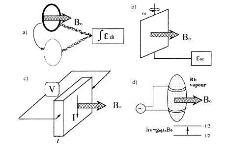
Figure 4.11. Several methods for measuring magnetic fields: (a) search coil fluxmeter, (b) rotating coil fluxmeter, (c) Hall probe and (d) nuclear magnetic resonance probe.
Force Methods
In the Faraday balance, the sample is subjected to a non - uniform horizontal field \(\boldsymbol{B}_{0}\), which has a gradient \(\partial B_{x}/\partial z\) in the vertical, \(z\) direction (figure 4.12(a)). The force on a sample of moment \(m\) is given by (1.12)
\(\boldsymbol{F}=\nabla(\boldsymbol{m}\cdot\boldsymbol{B}_{0})=m(\partial B_{x}/\partial z)\boldsymbol{e}_{z}\) (4.11)
where \(B_{0}=\mu_{0}H\). Hence, measurement of the force on a sample freely suspended from a sensitive balance gives \(m(\partial B_{x}/\partial z)\). When the field gradient is generated by an electromagnet with shaped pole pieces, the method is insensitive in zero field, and \(\partial B_{x}/\partial z = cB_{x}\), where the constant \(c\) is determined by the shape of the pole pieces. The Faraday balance in its basic form is useless for studying permanent magnets because it cannot measure remanence, but this defect can be overcome if an electromagnet or permanent magnet flux source is used to generate a uniform field and the field gradient is produced independently by a set of gradient coils or a small permanent magnet array. The Faraday balance requires calibration with a standard sample and a sensitivity of the order of \(10^{-6}\ J\ T^{-1}\ [10^{-3}\ emu]\) is typical. From (4.11), this corresponds to the force equivalent of a moment of \(0.1\ mg\) with a field gradient of \(1\ T\ m^{-1}\). Thermomagnetic analysis (TMA) involves a simple magnetic balance, where the force on a sample in a field gradient produced by a permanent magnet is recorded, as temperature
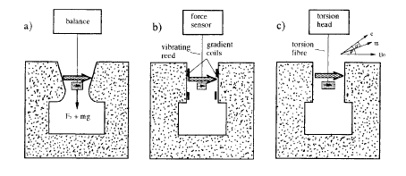
Figure 4.12. Force methods of measuring a sample in the horizontal field of an electromagnet: (a) the Faraday method; (b) the alternating gradient force method; (c) the torque method.
is ramped by means of a miniature furnace; TMA is used to measure the Curie temperature(s) of the magnetic phase(s) present.
The sensitivity of any measurement with a continuous analogue output can be enhanced if the continuous signal is converted to an alternating signal at a fixed frequency which is then sensed using a lock - in amplifier tuned to that reference. The alternating gradient force magnetometer (AGFM) is an ac version of the force magnetometer. An alternating field gradient is applied in the horizontal direction at a frequency which may be chosen to coincide with the resonant frequency of the sample support rod, a vertical vibrating reed. The applied field is uniform and horizontal (figure 4.12(b)). The sensitivity of the measurement is thereby increased by some orders of magnitude to \(10^{-11}\ J\ T^{-1}\ [10^{-8}\ emu]\), which makes it possible to measure small pieces of ferromagnetic films a few nanometres in thickness.
In the torque magnetometer, a disc - shaped, cylindrical or spherical specimen of a single - crystal or oriented magnet is suspended perpendicular to an axis of symmetry from a vertical fibre in a horizontal magnetic field (figure 4.12(c)). The torque \(\Gamma\) on the specimen is measured as the field is rotated in a horizontal plane. The instrument measures anisotropy, not magnetization. If the field is at an angle \(\phi\) to the easy axis, as shown in the figure, then \(E = E_{\mathrm{a}}-M B_{0}V\cos(\phi-\theta)\) where the anisotropy energy \(E_{\mathrm{a}}\) is given by (3.3), for example. In equilibrium, \(\partial E/\partial\theta = 0\), hence \(\partial E_{\mathrm{a}}/\partial\theta = M B_{0}V\sin(\phi - \theta)\). This term is identified as the torque of the sample hence
\(\Gamma/V=-\partial E_{\mathrm{a}}/\partial\theta\) (4.12)
The shape of the torque curve reflects the symmetry of the crystal; for example, if \(E_{\mathrm{a}}=K_{1}V\sin^{2}\theta\), \(\Gamma=-K_{1}V\sin2\theta\) and \(K_{1}\) can be deduced from the magnitude of the torque oscillations. Sensitivity is typically \(10^{-13}\ N\ m\). For accuracy, the
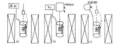
Figure 4.13. Flux methods of measuring magnetization of a sample in the vertical field of a superconducting magnet: (a) extraction, (b) vibrating - sample magnetometer and (c) SQUID magnetometer.
applied field should exceed the anisotropy field and be sufficient to saturate the sample and make \((\phi-\theta)\) a small angle. This is impractical for many hard magnets and anisotropy constants are then better deduced from the high - field magnetization curves (figure 4.14).
Flux Methods
The simplest method of measuring magnetization based on the change of flux through a coil is the extraction method where a sample positioned at the centre of a coil in the field is quickly removed to a point far from the coil (figure 4.13(a)). The change of flux threaded the coil is obtained by integrating the induced emf, (4.10), just as for a search coil. The magnetic moment of the sample is proportional to the change of flux registered on the fluxmeter. An improved pick - up coil is composed of two oppositely wound segments, so changes of applied field do not register. The sensitivity of an extraction magnetometer is typically \(10^{-8}\ J\ T^{-1}\).
The ac version of the extraction method is the vibrating - sample magnetometer (VSM), named the Foner balance after its inventor (Foner 1962). Here the sample is mounted on a vertical rod and vibrated vertically in the vicinity of a set of pick - up coils (figure 4.13(b)). The coil arrangement depends on whether the applied field is vertical, as with a superconducting solenoid, or horizontal, as with an electromagnet. In either case, the upper and lower coils (pairs of coils for the horizontal applied field) are oppositely wound so that the emfs induced in them by the vibrating sample add. Two pairs of coils are used in a quadrupole configuration for the horizontal applied field to create a saddle point around which the sensitivity is independent of sample position. The vibration frequency is typically in the range 10 - 100 Hz and the vibration
Table 4.6. Comparison of methods for measuring magnetization and hysteresis of permanent magnet materials [1 J T⁻¹ = 1 A m² = 1000 emu].
| Method | Open/closed circuit | Typical sensitivity (J T⁻¹) |
|---|---|---|
| Faraday | Open | 10⁻⁶ |
| Alternating gradient force | Open | 10⁻¹¹ |
| Extraction | Open | 10⁻⁸ |
| Vibrating sample | Open | 10⁻⁸ |
| SQUID | Open | 10⁻¹¹ |
| Hysteresisgraph | Closed | 10⁻⁴ |
amplitude of a few tenths of a millimetre is controlled by a feedback loop. The sensitivity of a well - designed VSM is better than \(10^{-8}\ J\ T^{-1}\). By using a double set of pick - up coils at right angles to each other, the magnetization vector in the horizontal plane can be recorded and resolved into components \(m_{\theta}\) and \(m_{\perp}\). If the sample or the field is rotated, the quantity \(m_{\perp}B_{0}\) can be deduced; this is equal to \(\Gamma\) and yields \(\partial E_{\mathrm{a}}/\partial\theta\) from (4.12).
An extremely sensitive way of measuring the flux change through a pick - up coil is with a superconducting quantum interference device (SQUID). The flux threading the superconducting circuit is a constant, hence current will flow in a pick - up coil made of superconducting wire to compensate whatever flux change occurs when the sample is extracted from it (figure 4.13(c)). Part of the circuit acts as a transformer to couple some flux into the active area of the SQUID. Great sensitivity is possible, because the device can respond to a fraction of a flux quantum (\(\Phi_{0}=h/2e = 2.068\times10^{-15}\ T\ m^{2}\)), but the measurement is time consuming as it involves an extraction at each point and it is necessary to change the field in the superconducting magnet from one measuring point to the next on the hysteresis loop, which is slow. Methods of measuring magnetization and hysteresis are compared in table 4.6. Usually unnecessary in magnetization measurements on permanent magnets, where a 100 mg sample will have a moment of the order of \(10^{-2}\ J\ T^{-1}\ [10\ emu]\). More important is the ability to saturate the magnetization and measure a major hysteresis loop quickly. The VSM is often the best choice, operating with an electromagnet or a permanent - magnet flux source for measurements on alnicos and hard ferrites, and with a superconducting magnet for measurements on rare - earth magnets.
High sensitivity is needed for very small samples such as thin films or tiny crystallites comparable in size to the critical single - domain size \(R_{\mathrm{sd}}\) where sample mass may be smaller than 1 \(\mu g\). Also, magnetic viscosity measurements, where small changes of magnetization in the second quadrant of the hysteresis
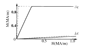
Figure 4.14. Magnetization curves of a crystal of \(YCo_{5}\) measured parallel and perpendicular to the \(c -\)axis. The data are plotted as a function of the external field (full lines) or the internal field (dotted line) after correction for the demagnetizing field.
loop are recorded as a function of time, require great stability and sensitivity. The SQUID is then the best choice.
As an example of a magnetization measurement, data on an oriented spherical crystal of hexagonal \(YCo_{5}\) which has easy - axis anisotropy shown in figure 4.14. Measurements are made for the field applied parallel and perpendicular to the easy axis. In the parallel direction, an external field \(H = M_{\mathrm{s}}/3\) equal to the maximum demagnetizing field is required to achieve saturation. The curves shown by dotted lines have been corrected for the demagnetizing effect and they are plotted as a function of \(H'=H - DM\), where \(D = 1/3\). The perpendicular magnetization curve is practically linear for this compound and it reaches saturation when the value of the internal field \(H'\) reaches that of the anisotropy field \(H_{\mathrm{a}}=2K_{1}/\mu_{0}M_{\mathrm{s}}\), where \(K_{1}\) is the first anisotropy constant. There is no high - field slope because \(YCo_{5}\), like cobalt, is a strong ferromagnet. Further examples of magnetization curves are to be seen in chapter 5.
When the second anisotropy constant \(K_{2}\) is non - negligible, the perpendicular magnetization curve is curved. Both constants can be deduced from the Sucksmith - Thompson (1954) plot of \(H/M\) versus \(M^{2}\) (problem 4.10).
A direct measurement of the saturation field \(H_{\mathrm{s}}\) is possible in a short - pulse field using the singular - point detection (SPD) technique. The saturation field \(H_{\mathrm{s}}\) is equal to \(H_{0}\) when \(K_{2}=K_{3}=0\). Otherwise \(H_{\mathrm{s}}\) is \((2K_{1}+2K_{2}+3K_{3})/\mu_{0}M_{\mathrm{s}}\) (section 3.2.3.2). The SPD method involves differentiating the signal in a pick - up coil around the sample so that \(\mathrm{d}V/\mathrm{d}t\) is recorded during the pulse. The derivative \(\mathrm{d}B/\mathrm{d}t\) is simultaneously recorded using a search coil so that the field \(H_{\mathrm{s}}\) at which a singularity appears in the second derivative of the magnetization curve can be determined.
Susceptibility
Susceptibility may be deduced from the slope of the magnetization curve, generally measured in an open circuit. When the sample mass is known, it is convenient to deduce \(\kappa\), in J T⁻² kg⁻¹ where \(\kappa=\sigma/B_{0}=M/(\rho B_{0})\). Otherwise, if the volume or density of the sample is known, the dimensionless susceptibility \(\chi\) defined by \(M = \chi H\) can be obtained directly. (The cgs susceptibility is smaller by a factor \(4\pi\).) The high - field susceptibility in the ferromagnetic state may be read from the slope of the magnetization curve beyond technical saturation. Values for iron - based alloys are about \(10^{-3}\). The paramagnetic susceptibility above the Curie point may be used to deduce the Curie constant \(C\) and the paramagnetic Curie temperature \(\theta_{\mathrm{p}}\) if the data follow a Curie - Weiss law \(\chi = C/(T-\theta_{\mathrm{p}})\). The effective local moment is
\(m_{\mathrm{eff}}=(3k_{\mathrm{B}}C_{\mathrm{m}}/\mu_{0}N_{\mathrm{A}})^{1/2}\) (4.13)
where \(C_{\mathrm{m}}\) is the molar Curie constant, \(N_{\mathrm{A}}\) is the number of atoms in a mole and \(m_{\mathrm{eff}} = p_{\mathrm{eff}}\mu_{\mathrm{B}}\). \(C_{\mathrm{m}}\) is related to \(p_{\mathrm{eff}}\) by \(C_{\mathrm{m}} = 1.571\times10^{-6}p_{\mathrm{eff}}^{2}\ [0.125p_{\mathrm{eff}}^{2}\) in cgs units].
As discussed in chapter 2, the Pauli paramagnetic susceptibility is of the order of \(\alpha^{2}\) (about \(6\times10^{-5}\)). Above \(T_{\mathrm{C}}\), moment formation in the paramagnetic state greatly enhances this value and leads to the divergence of \(\chi\) at \(T_{\mathrm{C}}\).
In ac susceptibility measurements, the initial susceptibility \(\chi_{i}\) is determined by applying a small low - frequency alternating field of about \(1 - 1000\ A\ m^{-1}\). A pair of precisely balanced concentric and coaxial pick - up coils is used together with a driving coil to generate the field, so that no emf is induced in the absence of a sample. High sensitivity is achieved by using a lock - in amplifier to detect the emf in the pick - up coil containing the sample; the real and imaginary parts of the ac susceptibility \(\chi=\chi'+i\chi''\) are deduced from the components of the signal in phase and in quadrature with the driving field \(H\). In aligned magnets, \(\chi_{i}\) is quite different when measured parallel or perpendicular to the alignment direction, which is the easy - axis of the crystallites. The real part of the perpendicular susceptibility \(\chi_{\perp}'=\mu_{0}M_{\mathrm{s}}^{2}/2K_{1}\) is due to magnetization rotation, but the parallel susceptibility \(\chi_{\parallel}'\) is governed by reversible domain - wall motion, and it will be different in the virgin and in the remanent states. The imaginary part of the susceptibility \(\chi''\) is dominated by irreversible wall motion. Ac susceptibility is often used to determine Curie temperatures and locate other magnetic phase transitions. As \(\chi'\) diverges at \(T_{\mathrm{C}}\) the maximum value actually measured is limited to \(1/D\) by the demagnetizing field.
Measurements of \(T_{\mathrm{C}}\) are used to estimate the exchange constant \(\mathcal{J}_{0}\) from (2.124) and \(A\) from (3.61). When more than one exchange constant interaction is involved, or if \(\mathcal{J}_{0}\) is antiferromagnetic, \(\theta_{\mathrm{p}}\) is different from \(T_{\mathrm{C}}\), as discussed in section 2.3.2.
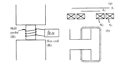
Figure 4.15. Schematic illustration of the hysteresisgraph for measuring \(B\) or \(M\) as a function of the internal field \(H'\) (left). The insets show a compensated coil used to measure \(M\) (a) and potential coils used to measure \(H'\) (b).
Closed Circuit Magnetization Measurements: Precision and Insights
For closed - circuit measurements, the material is usually in the form of a block or cylinder with uniform cross - section and parallel faces. It is clamped between the poles of an electromagnet so that it closes a magnetic circuit, like that shown in figure 4.23. There is therefore no need for a demagnetizing correction, as \(H'=H - DM\) equals the external field. The instrument in figure 4.15, known as a hysteresisgraph or permeameter, is designed to measure \(B(H)\) loops where \(H\) is the internal field in the sample. For materials which cannot be saturated in the field of a pulsed electromagnet (about \(2\ T\)), the sample may be first saturated along its axis in a pulsed field and then transferred to the hysteresisgraph for measurement of the demagnetizing curve in the second quadrant. Various arrangements of coils and sensors are available to measure \(B\), \(M\) (or \(J=\mu_{0}M\)) and \(H\). \(B\) can be measured by winding a coil of \(n\) turns of fine wire around the centre of the sample and bringing the leads to a fluxmeter as a tightly twisted pair. The fluxmeter is effectively an integrating voltmeter. The cross - section of the coil is practically the same as that of the magnet, \(A_{\mathrm{m}}\), and the fluxmeter integrates \(-N A_{\mathrm{g}}(\mathrm{d}\Phi/\mathrm{d}t)\). The \(H\) - sample, as shown in figure 4.15, has the pole - piece in the air - gap close to the magnet, so as to measure using a small Hall probe placed opposite the pole - piece. \(H_{\mathrm{f}}\) is continuously at the interface (figure 2.10). Alternately, a small search coil may be located in the air - gap and connected to a second fluxmeter. The field in the electromagnet is swept, and \(B\) and \(H\) are recorded on a chart recorder or on a computer.
An alternative coil arrangement is used to measure the magnetization \(M\). It consists of two concentric circular flat windings having areas \(A_{1}\)
with \(N_{1}\) turns and \(A_{2}\) with \(N_{2}\) turns. The induced emf is proportional to \(N_{1}[(A_{1}-A_{\mathrm{m}})\mu_{0}H + A_{\mathrm{m}}B]-N_{2}[(A_{2}-A_{\mathrm{m}})\mu_{0}H + A_{\mathrm{m}}B]\). If the dimensions of the two coils are chosen so that \(N_{1}A_{1}=N_{2}A_{2}\), the emf is proportional to \((N_{1}-N_{2})A_{\mathrm{m}}(B - \mu_{0}H)=(N_{1}-N_{2})A_{\mathrm{m}}\mu_{0}M\). The induced emf can therefore be integrated on the fluxmeter to give magnetization directly.
When the pole pieces of the electromagnet approach saturation, the \(H\) field is distorted in the vicinity of the sample. The measurement of \(H\) at a spot in the airgap adjacent to the sample can then give erroneous readings. The field can then be deduced from the magnetic potential difference \(\Delta\varphi_{\mathrm{m}}=\int H\mathrm{d}l\) between the two ends of the magnet using a technique known as a potentiometer. This is a long flexible coil of small cross - sectional area \(A\), evenly wound with \(n\) turns per metre of fine wire. It is connected to a fluxmeter, with one end fixed, and the change of flux measured as the free end is moved from one point to another (figure 4.24).
Applying Ampère's law \(\oint H\mathrm{d}l = 0\) to a loop running down the centre of the coil with an arbitrary return path including no current - carrying conductors, we find \(\int H\mathrm{d}l=\varphi_{\mathrm{s}}-\varphi_{\mathrm{e}}\) where \(A\) and \(B\) are points at the ends of the coil. Since the path of the first integral runs along the centre of the coil, it can be related to the flux \(\Phi=\mu_{0}nAI\). So
\[\Phi=\mu_{0}nA(\varphi_{\mathrm{s}} - \varphi_{\mathrm{e}})\] (4.14)
the coil measures \(\Delta\varphi_{\mathrm{m}}\) between two points when it is first connected to a fluxmeter and brought up into the vicinity of the magnet with its ends placed at the two points. The potential coil may be split into two parts and the ends embedded in the poles of an electromagnet, as shown in figure 4.15(b). The two ends of a potential coil connected to the fluxmeter are analogous to the two voltage probes connected to a voltmeter for normal electrical measurements. A magnet can be regarded as a source of magnetomotive force, rather like a battery which is a source of electromotive force. The analogy between magnetic and electric circuits, though not exact, is quite useful. It is developed in section 4.3.
The accuracy of \(B(H)\) measurements, with periodic calibration of the fluxmeter, is of the order of \(1\%\).
Domain Observation: Visualizing Magnetic Structuresn
Techniques for visualizing domains and domain walls have been developed which depend on sensing the stray field \(H\) outside the magnetic material, or the magnetization \(M\) or flux density \(B\) inside it. The specimen has to be prepared as a polished surface, foil or thin film which begs the question of whether the domains observed at the surface are actually representative of the bulk. Bulk domains can be sensed using specialized methods such as neutron tomography or small - angle neutron scattering. Nevertheless much useful information regarding the microscopic parameters \(A\) and \(K_{1}\) can be obtained
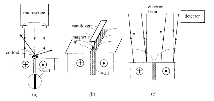
Figure 4.16. Stray - field methods of domain observation: (a) the Bitter method, (b) magnetic force microscopy and (c) scanning electron microscopy.
from domain studies, and insight into coercivity mechanisms and magnetization reversal is achieved by simultaneous observation of the domain structure and microstructure.
Stray - Field Methods
The first method to be developed for visualizing domains in the 1930s was the Bitter method (Bitter 1931) (figure 4.16). A magnetic colloid, normally a drop of oil - water - based ferrofluid, is spread over the polished surface of the sample and the tiny ferromagnetic particles are drawn to the regions of maximum field gradient, thereby decorating the domain walls. Magnetic force microscopy (MFM) is a scanning probe technique which is based on the same principle. A ferromagnetic tip mounted on a tiny cantilever or a silicon cantilever coated with a ferromagnetic film is rastered across the surface of the sample and the force derivative registered by the deflection of the cantilever or the change of its mechanical resonance frequency gives an image of a stray - field gradient at the surface. Reading magnetically recorded information from disks or tapes likewise depends on sensing the stray - field distribution of the domain pattern imposed on the magnetic medium, using an inductive or magnetoresistive pick - up head (cf figure 6.14).
Scanning electron microscopy (SEM) is a common method in materials science which involves rastering a sample surface with a finely focused electron beam and detecting the secondary electrons emitted from the surface. It is used to image both microstructure and topology, and can provide chemical analysis on a local scale because the energies of the secondary electrons and especially
those of the accompanying x - rays are characteristic of the chemical elements present. Sensitivity is good for elements with 3s and deeper electronic shells (Na and beyond). Lower - energy x - rays from light elements can be observed with a special window detector. SEM can be adapted to provide magnetic contrast by detecting the deflection of the secondary electrons in the stray field produced near the surface of a multidomain sample. Alternatively, the spin polarization of the secondary electrons can be monitored as the electron beam is rastered across the surface; this technique is known as scanning electron microscopy with polarization analysis (SEMPA).
Magneto - Optic and Electron -Optic Methods
The principle of the second group of domain - imaging techniques is that a beam of radiation passing through a solid is influenced in some way by the ferromagnetic order of the solid. In the case of electromagnetic radiation, the magneto - optic effects depend on the magnetization \(M(\boldsymbol{r})\), whereas if an electron beam is used in transmission electron microscopy (TEM) the interaction depends on the Lorentz force and the relevant quantity is the local flux density \(B(\boldsymbol{r})\).
A steady magnetic field has no influence on electromagnetic waves in free space, but light in a medium interacts with the magnetization of electrons in matter via the spin - orbit interaction. The effects are weak, but tend to be more pronounced in heavy atoms (see table 3.4). In general, the magneto - optic effects are derived from the complex dielectric tensor \(\varepsilon_{ij}\), defined by the relation \(D_{i}=\varepsilon_{ij}E_{j}\). Neglecting the optical activity of the unmagnetized crystal and assuming \(\boldsymbol{K}\) propagates along the \(z\) - direction, one obtains the antisymmetric tensor
\(\begin{pmatrix} \varepsilon_{xx}&\varepsilon_{xy}&0\\ -\varepsilon_{xy}&\varepsilon_{yy}&0\\ 0&0&\varepsilon_{zz} \end{pmatrix}\) (4.15)
An interpretation of the off - diagonal matrix elements is that the magnetic field \(\boldsymbol{H}\) in the electromagnetic wave gives rise to a Lorentz force \(-\mu_{0}e(\boldsymbol{v}\times\boldsymbol{H})\) which mixes the \(x\) and \(y\) components of the electron's motion. In ferromagnets with quenched orbital momentum, it is not possible to distinguish between clockwise and anticlockwise electron motion, and \(\varepsilon_{xx}=\varepsilon_{yy}\). However, the spin - orbit interaction restores an orbital moment and leads to magnetic dichroism or Faraday and Kerr rotation (figure 4.17).
Magneto - optic effects may be observed in transmission or reflection. When plane - polarized light passes through a transparent ferromagnetic medium with its wavevector \(\boldsymbol{K}\) parallel to the direction of magnetization, the plane of polarization is observed to rotate by an amount proportional to the path length in the magnetic medium. This is the Faraday effect and its discovery was the first hint of a link between light and magnetism. The effect is due to magnetic circular birefringence; the linearly polarized light may be decomposed into two circularly rotating circularly polarized beams which travel with slightly different
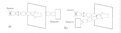
Figure 4.17. Magneto - optic effects: (a) the Faraday effect and (b) the polar Kerr effect.
velocities. The resulting phase difference between them causes the plane of polarization to rotate through an angle \(\theta_{\mathrm{F}}=V_{\mathrm{F}}(\boldsymbol{K})\int\boldsymbol{M}\cdot\mathrm{d}\boldsymbol{l}\) where \(V_{\mathrm{F}}(\boldsymbol{K})\) is the Verdet constant of the material which is a function of wavelength \(\lambda = 2\pi/K\). The Faraday effect is non - reciprocal in the sense that the rotation (clockwise or counterclockwise) depends on whether the wavevector \(\boldsymbol{K}\) of light is parallel or antiparallel to \(\boldsymbol{M}\). Hence, Faraday rotation is cumulative; as light is reflected back along its path in a ferromagnetic medium, the resultant rotation is twice that for a single pass, not zero.
Magnetic circular dichroism is a related effect, where the absorption coefficients for left - and right - circularly polarized light are slightly different. This has the effect of transforming the linearly polarized incident beam into an elliptically polarized transmitted beam.
The Faraday spectrum for a film of \(\text{BaFe}_{12}\text{O}_{19}\) is shown in figure 4.18. The effect is greatest in the vicinity of the transitions involving the \(\text{Fe}^{3 + }\) magnetic ions and is enhanced near the absorption edge. Typical values of \(V_{\mathrm{F}}\) are \(10^{2}\) radians m⁻¹. A useful figure of merit is the product \(V_{\mathrm{F}}l_{\mathrm{a}}\) where \(l_{\mathrm{a}}\) is the absorption length, the thickness of material which will reduce the intensity of the transmitted beam by a factor e.
The polar Kerr effect is the analogue in reflection of the Faraday effect. A beam of plane - polarized light is reflected from the surface of a ferromagnetic material with the plane of polarization rotated through a small angle \(\theta_{\mathrm{K}}\) of order \(0.1^{\circ}\). The Kerr rotation for a metal is similar in magnitude to the Faraday rotation on transmission through a film of the metal thin enough to be transparent. In magneto - optic recording media, the effect is optimized with dielectric coatings. Multiple reflections take place from the top and bottom surface of the film. The Kerr microscope, a metallographic microscope modified to incorporate precise polarization analysis, will give simultaneous images of the microstructure and the domain structure. The picture in figure 4.19 shows domains in the crystallites of an unmagnetized sintered Nd - Fe - B magnet, where the crystallite size is larger than \(2R_{\text{sd}}\).
Both Faraday and Kerr effects can also be used to investigate magnetization processes. When the light beam is much larger than the domain size, initial magnetization curves and hysteresis loops reflecting the net magnetization are
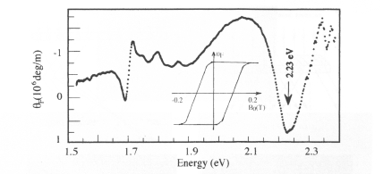
Figure 4.18. The Faraday effect spectrum for \(\text{BaFe}_{12}\text{O}_{19}\) at 20 K. The inset shows a hysteresis loop for the film obtained with light of wavelength 633 nm. (After Masterson et al 1997.)
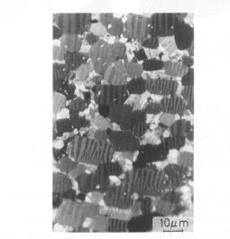
Figure 4.19. An image of the polished surface of an Nd - Fe - B sintered magnet in the Kerr microscope. The magnet is in the virgin state and the oriented \(\text{Nd}_{2}\text{Fe}_{14}\text{B}\) crystallites are unmagnetized multidomains. The weak domain contrast is due to Kerr rotation observed between crossed polarizers. (Photograph courtesy of H Krommüller.)
obtained. The techniques are very sensitive and have been used to investigate films as little as a monolayer thick. However, they do not give the absolute value of \(M\) and are difficult to calibrate.
In addition to the polar Kerr and Faraday effects, there exist a number of other magneto - optic techniques where the intensity or phase of the polarized
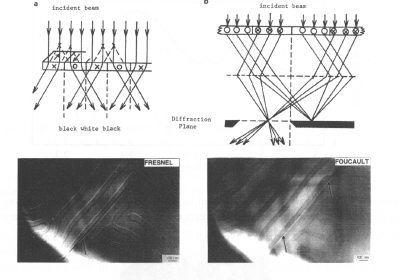
Figure 4.20. Imaging schemes in TEM: (a) a Fresnel image and (b) a Foucault image. The examples are \(\text{Nd}_{2}\text{Fe}_{14}\text{B}\). (Courtesy, J. Fidler.)
Light is influenced by the magnetization. In the transverse Kerr effect, for example, a difference in intensity in the reflected beams polarized perpendicular and parallel to the magnetization is observed when \(M\) lies in the plane of the sample (linear magnetic dichroism). The transverse Kerr effect is useful for studying magnetization processes and domain structure in the plane of a magnetic film.
An important group of domain - observation techniques is based on transmission electron microscopy (TEM). The electron experience a Lorentz force \(-e\boldsymbol{v}\times\boldsymbol{B}\) as they pass through a magnetized sample and so they are deflected unless \(\boldsymbol{B}\) is parallel to their direction of motion. Two methods of obtaining magnetic contrast in Lorentz microscopy are the Fresnel scheme and the Foucault scheme sketched in figure 4.20. The former images the domain walls and the latter the domains. One problem, however, is that there is usually a magnetic field at the sample in a standard electron microscope due to the focusing lens and this field will obviously perturb the domain structure. Instruments with special lenses have been developed to facilitate imaging of domains in specimens subject to almost no magnetic field. A feature of Lorentz microscopy is the very high spatial resolution obtainable. Figure 4.21 shows domain walls on a nanometre scale in a nanocrystalline Nd - Fe - B alloy prepared by melt spinning. A major drawback of the method is the need to prepare the samples in the form of foils thin enough for electrons to traverse.


