

2.Understanding Basic Magnetism: An Overview
This chapter gives an introduction into the physical ideas on which our understanding of permanent magnetism is based. Besides fundamental phenomena, such as spin-orbit coupling and ionic magnetism, the key issue is the microscopic origin of magnetization M(r) in solids, that is the formation of atomic spin and orbital momenta as well as finite-temperature inter-atomic ordering. Since there are different ways of realizing moment formation and magnetic order in permanent magnets, some emphasis is put on the distinction between 3d oxides, 3d metals and rare-earth intermetallics.
Readers primarily interested in materials and applications rather than the basic physics may use this chapter as a reference source without working their way through all the mathematical details. Although a thorough and comprehensive discussion is attempted, it has not been possible to cover areas only peripherally related to permanent magnets, such as thin-film magnetism and magnetic properties of superconductors. The problems and exercises at the end of the chapter will serve to fill out some details missing in the concise presentation.
2.1 Fields and Interactions
Fields and Interactions in Basic Magnetism: Key Insights
Magnetism involves both atomic-scale electrostatic interactions and long-range magnetostatic dipole interactions. Equation (1.2) shows that the magnetic dipolar field Hdm created by a solid can be written as a superposition of atomic dipolar fields created by the magnetization distribution M(r). However, this is only one part of the problem since the dependence of the magnetization M on the external magnetic field H has to be specified from the solid's electronic structure. On the one hand, there are one-electron interactions ultimately derived from the relativistic Dirac equation, which includes electrostatic. Zeeman and spin-orbit interactions on a quantum-mechanical level. On the other hand, one has to take into account electrostatic many-body interactions such as inter-atomic exchange. The aim of this section is to present some fundamental topics, electromagnetism, angular momentum algebra, spin-orbit coupling, exchange and magnetostatics rather than to investigate particular aspects of permanent magnetism.
Electromagnetic Fields: Foundations of Magnetisms
Electromagnetic fields created by atomic matter obey the relativistic, space-time symmetric Maxwell equations. First, we separate the electro-dynamic aspect of magnetism from its atomic origin by formulating the magnetostatic equations in terms of dipolar fields.
Maxwell's Equations
Electric and magnetic fields are not independent but obey the four famous equations
\(\text{curl } H' = j(r) + \frac{\partial D}{\partial t}\) \(\text{curl } E' = -\frac{\partial B}{\partial t}\) (2.1a, b)
\(\text{div } B = 0\) \(\text{div } D = \rho(r)\) (2.2a, b)
where \(j\) is the electric current density. The total electric and magnetic field strengths \(E'(r,t)\) and \(H'(r,t)\) and the respective flux densities \(B(r,t)\) and \(D(r,t)\) obey the equations of state1
\(B = B(H',...)\) \(D = D(E',...)\) (2.3)
where... denotes other variables, such as time and pressure. The vacuum relations \(D = \epsilon_0 E'\) and \(B = \mu_0 H'\) make it convenient to rewrite (2.3) as
\(B = \mu_0 H' + J(H',...)\) \(D = \epsilon_0 E' + P(E',...)\) (2.4)
where the magnetic polarization \(J\) (or the magnetization \(M = J/\mu_0\)) and the electric polarization \(P\) parameterize the magnetic and electric properties of a solid medium, respectively.
It must be emphasized that the functional form of (2.3) and (2.4) is not provided by Maxwell's equations but reflects the electronic structure of the material, which has to be determined separately. In general, the nonlinear equations of state \(M = M(H')\) and \(P = P(E')\) exhibit hysteresis and cannot be approximated by linear relations such as \(M = \chi H\), where \(\chi\) is the magnetic susceptibility. The reason for magnetic hysteresis is that the magnetization cannot follow the magnetic field instantaneously when there are magnetic energy barriers associated with the microstructure of the solid.
1 Equations of state (materials equations) describe the response of a physical system to an external force.
Continuum Magnetostatics
Maxwell's equations describe phenomena such as light propagation, electromagnetic induction and magnetic flux creation by solenoids, as well as permanent magnetism. As we will see in section 3.1, electrostatic interactions are necessary to explain atomic-scale magnetic order and anisotropy, but charge neutrality in magnetostatics causes \(E\) and \(D\) to be negligible on a macroscopic scale. Furthermore, when considering permanent magnetism it is reasonable to ignore high-frequency electromagnetic contributions. In the absence of electric currents and time-varying fields Maxwell's equations reduce to the magnetostatic equations (1.4b), which can be written in integral form as
\(\int B \cdot dS = 0\) and \(\oint H' \cdot dl = 0.\) (2.5)
In addition, there is the equation of state \(B = B(H').
Although the two equations (2.5) epitomize continuum magnetostatics, they are not very well adapted to atomic physics. The reason is that the magnetic flux \(B = \mu_0(H' + M)\) has the very inconvenient functional structure \(B = \mu_0H + \mu_0H_{dm}(M) + \mu_0M\) where the magnetization \(M\) exhibits a complicated dependence on the external field (figure 1.1). To solve the magnetostatic equations we introduce the magnetostatic potential \(\varphi_m\) defined by \(H' = -\nabla\varphi_m\). This potential satisfies \(\nabla \times H' = 0\) and, with \(\nabla \cdot B = 0\), yields
\(\nabla^2\varphi_m = \nabla \cdot M.\) (2.6)
This is Poisson's equation, whose solution is known from electrostatics
\(\varphi_m(r) = -\frac{1}{4\pi} \int \frac{\nabla \cdot M(r')}{|r - r'|} dr' + \varphi_{ext}(r)\) (2.7)
where \(\varphi_{ext}\) is the potential of the external field. The total field (1.2) is therefore
\(H'(r) = -\frac{1}{4\pi} \int \frac{(r - r')\nabla \cdot M(r')}{|r - r'|^3} dr' + H.\) (2.8)
This equation ensures that the magnetostatic equations (2.5) are automatically satisfied and makes it possible to use \(M\) and \(H\) rather than \(B\) and \(H'\) to describe continuous magnetic solids. The continuum approximation assumes that \(M\) and \(H'\) are averaged over a few atomic distances (figure 2.1).
Figure 2.2 shows how monopole fields would impose yield dipolar fields (1.3). The dipolar character of magnetic fields follows from the non-existence of magnetic monopoles, that is from \(\nabla \cdot B = 0\). Nevertheless, (2.8)
2 The scalar-potential representation is valid only in the absence of electric currents and time-varying electric fields. Otherwise one has to use the vector potential \(A\) (section 4.3.2).

Figure 2.1. Atomic dipole moments \(m_i\) (arrows) determine the local magnetization \(M(r) = \delta(\sum m_i)/\delta V\). \(e\) is a unit vector.
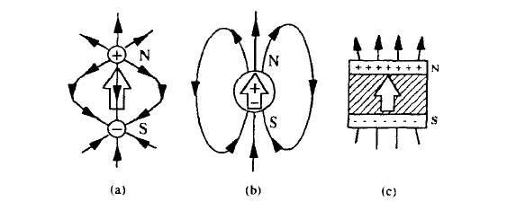
Figure 2.2. Superposition of monopole fields (a) yielding a dipole field (b). Homogeneously magnetized blocks exhibit surface poles (c). The magnetic-moment vector is represented by a hollow arrow.
means that \(H_{dm} = H' - H\) may be written as
\(H_{dm}(r) = -\frac{1}{4\pi} \int_{V'} \frac{\nabla \cdot M(r')(r - r')}{|r - r'|^3} dr' + \frac{1}{4\pi} \int_{S'} \frac{(r - r')}{|r - r'|^3} M(r') \cdot dS'\) (2.9)
where bulk and surface contributions are separated. The first integral may be interpreted as the field due to a fictitious magnetic charge density \(\rho_m(r) = -\nabla \cdot M\) throughout the bulk of the sample. It is zero for a uniformly magnetized body. The second may be interpreted as the field due to a fictitious surface charge density \(\sigma_m(r) = M \cdot e_s\), where \(e_s\) is the unit vector normal to the surface. In practical calculations for block-shaped or cylindrical magnets it is customary to assume uniform magnetization and derive \(H_{dm}\) from the second term in (2.9).
The positive and negative magnetic charge density in equation (2.9) corresponds to the concept of north and south magnetic poles (N and S in figure 2.2). By definition, the \(H\) field goes from north to south, so that the tip of a moment vector indicates the magnetic north pole. The Earth is a confusing magnet, since its moment \(8 \times 10^{22} \text{ A m}^2\), corresponding to an average magnetization \(\mu_0 M = 0.09 \text{ mT}\), changes sign roughly every \(100000\) years. At the moment, the magnetic south pole is near the geographical north pole and vice versa. To avoid confusion it is advisable to eliminate north and south poles from the vocabulary of permanent magnetism, and to rely whenever it is convenient to do so on the fictitious surface charges. We will not refer to these poles again.
Quantum Theory of Atomic Magnetism Explained
Experiment shows that the motion of any particle of momentum \(p\) and energy \(E\) is wavelike, described by the wave vector \(k = 2\pi/\lambda = p/h\) and the circular frequency \(\omega = 2\pi f = E/h\). Planck's constant is very small, so that the wave character is not manifest on a macroscopic scale. The behaviour of atomic matter is reminiscent of vibrating strings, so that one has to use quantum-mechanical wave equations to describe interactions on an atomic level. Here we summarize some results of non-relativistic quantum mechanics.
The Schrödinger Equation
Solid-state magnetism arises from the motion of electrons which are subject to the attractive electrostatic potential \(V_0\) of the atomic nuclei. The starting point of non-relativistic quantum mechanics is the \(N\)-electron Hamiltonian:
\(\mathcal{H}(r_i, p_i) = \sum_{i} \frac{1}{2m_e} p_i^2 + V_{tot}(r_1, r_2, \ldots, r_N)\) (2.10)
where \(i = 1, \ldots, N\) and \(V_{tot} = V_0 + V_c\) is the total electrostatic potential, including the mutual Coulomb repulsion \(V_c\) of the electrons. Since \(p = m_e v\), where \(v\) is the electron velocity, the Hamiltonian (2.10) can be interpreted as the total energy of the electronic system.
Single particles behave as waves described by a wavefunction \(\psi = \psi_0 \exp(i\omega t - k \cdot r)\), where \(\omega = E/h\) and \(k = p/h\). It is appropriate to interpret \(E\) and \(p\) as operators acting on \(\psi\):
\(\mathcal{H} = i\hbar \frac{\partial}{\partial t}\) and \(\hat{p} = -i\hbar \frac{\partial}{\partial r}\). (2.11)
The eigenenergies and eigenfunctions we are seeking are obtained as stationary solutions of the time-dependent Schrödinger equation:
\(i\hbar \frac{\partial}{\partial t} \psi = \mathcal{H}(r, -i\hbar \frac{\partial}{\partial r}) \psi\). (2.12)
For the many-electron Hamiltonian (2.10) the Schrödinger equation is
\(i\hbar \frac{\partial \Psi}{\partial t} = -\frac{\hbar^2}{2m_e} \sum_{i} \nabla_i^2 \Psi + \sum_{i} V_0(r_i) \Psi + \sum_{ik} \frac{e^2}{8\pi \epsilon_0 |r_i - r_k|} \Psi\) (2.13)
where \(\Psi\) is the many-electron wavefunction, and the \(\nabla\) operator is defined as \(\nabla_i = e_i \partial / \partial x_i + e_j \partial / \partial y_i + e_z \partial / \partial z_i\) and \(e_i\), \(e_j\) and \(e_z\) are unit vectors. The indices \(i\) and \(k\) refer to the coordinates of the \(i\)th and \(k\)th electrons, respectively. If the Hamiltonian were a sum of one-electron Hamiltonians, then the ansatz \(\Psi(r_1, \ldots, r_N) = \psi(r_1) \psi(r_2) \ldots \psi(r_N)\) would decompose (2.13) into an set of independent differential equations. In fact, the third term, the mutual Coulomb repulsion of the electrons, makes such a separation impossible and introduces a considerable degree of complexity into the problem.
An approximate way of treating the mutual Coulomb repulsion is to introduce an effective (and generally spin-dependent) one-electron potential \(V(r)\). Separating the time dependence of \(\psi_0\) by putting \(\psi(r, t) = \psi_{\mu}(r) \exp(i E_{\mu} t / \hbar)\) yields the stationary one-electron Schrödinger equation
\(E_{\mu} \psi_{\mu} = -\frac{\hbar^2}{2m_e} \nabla^2 \psi_{\mu} + V(r) \psi_{\mu}\) (2.14)
where the index \(\mu\) labels the one-electron eigenenergies \(E_{\mu}\) and eigenfunctions \(\psi_{\mu}\). This approach is particularly successful in metals, where the kinetic energy of the conduction electrons is much larger than their mutual Coulomb interaction (section 2.1.5). From the eigenfunctions of (2.14) we obtain the electronic charge density \(\rho_{el} = -e \psi_{\mu}^* \psi_{\mu}\) and of other operators \(\hat{A}\) their quantum-mechanical expectation values \(\langle A \rangle = \int \psi_{\mu}^* \hat{A} \psi_{\mu} dV\). From the electronic charge \(\int \rho_{el} dV = -e\) we see that \(\int \psi_{\mu}^* \psi_{\mu} dV = 1\), i.e., wavefunctions are usually normalized. It is always possible, and sometimes convenient, to interpret the operator \(\hat{A}\) as an \(N \times N\) matrix \(A_{ik}\). Here the indices \(i\) and \(k\) label the matrix elements, without any particular reference to electron coordinates, and the wavefunctions are \(N\)-component vectors \(\psi_i\).
Angular Motion and Magnetic Moment
The close relationship between the angular momentum \(m_{e}vR\) and the magnetic moment \(m\) of an electron leads to similar quantization rules for angular momenta and magnetic moments. The starting point are angular-momentum operators \(\hat{l}\) and \(\hat{s}\) acting on the electronic wavefunctions, where \(l\) refers to the orbital angular momentum and \(s\) to the spin angular momentum. Conventionally, small letters, such as \(l\), \(s\) and \(\psi\), denote the properties of independent electrons, whereas capital letters, such as \(\hat{L}\), \(\hat{S}\) and \(\Psi\), refer to many-electron systems. All these quantities are measured in \(J\) s, or often, in units of \(\hbar = 1.054 \times 10^{-34} \text{ J s}\). The eigenvalues and eigenfunctions of the angular momentum operators are classified by quantum numbers such as \(l\) and \(m\), which are dimensionless and must not be confused with angular-momentum operators or their expectation values.
A simple example is the in-plane rotation of a particle of mass \(m_p\) moving with velocity \(v\), the rigid free rotator. The kinetic energy \(E = m_pv^2/2\)
corresponds to a Hamiltonian written in terms of the angular momentum, \(\mathcal{H}(\phi, l_{z}) = l_{z}^{2} /\left(2 m_{p} R^{2}\right)\), where \(R\) is the distance from the axis of rotation and \(l_{z} = m_{p} v R\) is the angular momentum. The angular momentum operator is defined as \(\hat{l}_{z} = -i\hbar \partial / \partial \phi\), which yields the (time-independent) Schrödinger equation
\(E_{\mu} \psi_{\mu} = \frac{\hbar^{2}}{2 m_{p} R^{2}} \frac{\partial^{2} \psi_{\mu}}{\partial \phi^{2}}\). (2.15)
This equation is solved by the ansatz \(\psi_{\mu} = \exp(-i m_{\mu} \phi)\). Like amplitudes of vibrating strings, wavefunctions have to be continuous. This implies \(\psi_{\mu}(2 \pi) = \psi_{\mu}(0)\), so that the quantum number \(m_{\mu}\) must be an integer. The angular-momentum and energy eigenvalues are \(l_{z \mu}^{2} = -\hbar m_{\mu}\) and \(E_{\mu} = \hbar^{2} m_{\mu}^{2} /\left(2 m_{p} R^{2}\right)\). An important consequence of the quantization of angular momentum is the quantization of the orbital angular moment \(-\mu_{B} l_{z} = m_{\mu} \mu_{B}\).
Angular Momentum Algebra
The quantum mechanics of the spin and orbital angular momenta \(\hat{l}\), \(\hat{s}\), \(\hat{L}\) and \(\hat{S}\) is governed by angular-momentum algebra, which also applies to the total angular momenta \(\hat{j} = \hat{l} + \hat{s}\) and \(\hat{J} = \hat{L} + \hat{S}\) produced by spin-orbit coupling. Figure 2.3 illustrates the vector character of these quantities, which was not included in section 2.1.2.2. To derive the angular-momentum rules we start from the fact that the \(\phi\) dependence of any quantity can be expressed in terms of \(x\) and \(y\). Using the elementary identities \(\tan\phi = y/x\) and \(x^{2} + y^{2} = R^{2}\) we obtain \(\hat{l}_{z} = i\hbar(y\partial / \partial x - x\partial / \partial y)\). This result can be generalized to three-dimensional rotational motion
\(\hat{l} = i\hbar\left(z\frac{\partial}{\partial y} - y\frac{\partial}{\partial z}\right)e_{x} + i\hbar\left(x\frac{\partial}{\partial z} - z\frac{\partial}{\partial x}\right)e_{y} = i\hbar\left(y\frac{\partial}{\partial x} - x\frac{\partial}{\partial y}\right)e_{z}.\) (2.16)
The operator character of the orbital-momentum components leads to inequalities such as \((\hat{l}_{x}\hat{l}_{y} - \hat{l}_{y}\hat{l}_{x})\psi \neq 0\); in other words the components \(\hat{l}_{x}\), \(\hat{l}_{y}\) and \(\hat{l}_{z}\) of the orbital angular momentum \(\hat{l} = \hat{l}_{x}e_{x} + \hat{l}_{y}e_{y} + \hat{l}_{z}e_{z}\) do not commute. After some calculation we obtain the commutation relations \([\hat{l}_{x},\hat{l}_{y}] = i\hbar\hat{l}_{z}\), \([\hat{l}_{y},\hat{l}_{z}] = i\hbar\hat{l}_{x}\) and \([\hat{l}_{z},\hat{l}_{x}] = i\hbar\hat{l}_{y}\). A major consequence of this three-dimensional angular momentum algebra is that the average squared momentum \(\langle l^{2}\rangle = \hbar^{2}l(l + 1)\) exceeds its classical value \(\hbar^{2}l^{2}\), where \(l = \max\{m_{l}\}\) is another quantum number. There is never complete alignment of the orbital motion in the \(z\) direction, since the wave nature of matter yields some admixture of \(\hat{l}_{x}\) and \(\hat{l}_{y}\) character.
An explicit example of angular-momentum algebra is provided by Pauli's spin matrices \(\hat{\sigma}_{x}\), \(\hat{\sigma}_{y}\) and \(\hat{\sigma}_{z}\) appearing in the vector
\(\hat{\boldsymbol{\sigma}} = \begin{pmatrix}0 & 1 \\ 1 & 0\end{pmatrix}e_{x} + \begin{pmatrix}0 & -i \\ i & 0\end{pmatrix}e_{y} + \begin{pmatrix}1 & 0 \\ 0 & -1\end{pmatrix}e_{z}.\) (2.17)
It is easy to show the spin operator defined as \(\hat{s} = \hbar\hat{\boldsymbol{\sigma}}/2\) has eigenvalues \(s_{z} = \pm\hbar/2\) and obeys \(\langle s^{2}\rangle = 3\hbar^{2}/4\).
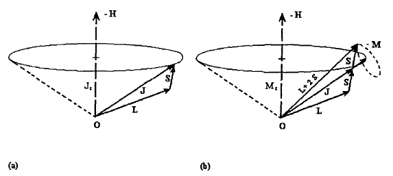
Figure 2.3. Vector model of the angular momentum: (a) total angular momentum and
(b) magnetic moment.
Exploring the Dirac Equation and Spin Moments
The kinetic energy \(m_{e}v^{2}/2\), on which (2.10) and (2.13) are based, indicates the non-relativistic character of the Schrödinger equation. In fact, the electronic spin and its interactions are relativistic phenomena. We have to construct a relativistic wave equation, the Dirac equation, which can, however, be recast as a Schrödinger equation in the limit of small relativistic corrections.
Space-time Symmetry
Both electromagnetism and mechanics can be described by space-time symmetric or relativistic equations. Newton's non-relativistic mechanics gives a reasonable description of most everyday phenomena, but there is no such non-relativistic limit in electromagnetism. Furthermore, we will see that the leading contribution to the magnetocrystalline anisotropy is a relativistic effect depending on the parameter \(v/c\), where \(v\) is the average electron velocity.
The simplest space-time symmetric electromagnetic phenomenon is the propagation of light: \(x^{2}+y^{2}+z^{2}-c^{2}t^{2}=0\). Introducing the four-dimensional space-time vector \(X=(x_{0},x_{1},x_{2},x_{3})=(ct,\mathbf{r})\), where the index \(0\) denotes the time coordinate, and a suitable scalar product the equation can be written as \(X\cdot X = 0\). One way of defining the four-vector scalar product \(X\cdot X\) is to multiply the time coordinate \(x_{0}\) by the imaginary unit \(i\), so that \(i^{2}=-1\) assures the right sign of the time contribution.
To show the space-time symmetry of the Maxwell equations we introduce the scalar and vector potentials \(\varphi_{e}\) and \(A\), respectively, which are defined by \(E = -\nabla\varphi_{e} - \partial A/\partial t\) and \(B = \text{curl }A\). Due to the identical vanishing of the operator products div curl and curl \(\nabla\) the homogeneous equations (2.1b) and (2.2a) are satisfied, so that only the inhomogeneous equations (2.1a) and (2.2b) remain. The potentials \(\varphi_e\) and \(A\) yield the four-vector potential \((\varphi_e, cA)\), from which \(E\) and \(H\) are obtained in the form of four-vector derivatives. The four-vector potential is obtained from the field sources \(\rho\) (charge density) and \(j\) (current density), which form the four-vector \((\rho, j/c)\).
Relativistic Energies
The classification of interaction phenomena according to their relativistic character is based on the kinetic energy
\(E = m_{e}c^{2}\sqrt{1 + \frac{v^{2}}{c^{2}}}\). (2.18)
The order of magnitude of the velocity of electrons in solids is \(\alpha c\), where \(\alpha = e^{2}/4\pi\epsilon_{0}\hbar c \approx 1/137\) is Sommerfeld's fine-structure constant. Expanding (2.18) into powers of \(v/c\) yields
\(E = m_{e}c^{2} + \frac{1}{2}\alpha^{2}m_{e}c^{2} - \frac{1}{8}\alpha^{4}m_{e}c^{2}\). (2.19)
Here \(m_{e}c^{2} = 0.511 \text{ MeV}\) is the rest energy of the electron, whereas electrostatic and magnetostatic energies scale as \(\alpha^{2}m_{e}c^{2}/2 = 13.6 \text{ eV}\) and \(\alpha^{4}m_{e}c^{2}/8 = 0.18 \text{ meV}\), respectively.
In inner shells, the velocity of the electrons is of the order of \(v = Z\alpha c\), where \(Z\) is the effective nuclear charge acting on the electrons. As a consequence, relativistic effects are enhanced in transition-metal and rare-earth ions. In particular, the pronounced relativistic spin-orbit coupling in rare-earth atoms is responsible for the strong magnetocrystalline anisotropy of rare-earth magnets.
Relativistic Quantum Mechanics
To describe relativistic phenomena in solids, we have to start from a space-time invariant electronic wave equation. Unfortunately, the Schrödinger equation
\(i\hbar\frac{\partial\psi}{\partial t} = -\frac{\hbar^{2}}{2m_{e}}\nabla^{2}\psi - e\varphi_{e}(r)\psi\) (2.20)
is non-relativistic, since the operators \(\partial/\partial t\) and \(\nabla = \partial/\partial r\) do not appear in the form of a space-time symmetric four-vector operator \(\partial/\partial X\). To find a relativistic wave equation we have to replace the expression \(\mathcal{H} = \hat{p}^{2}/2m\), on which Schrödinger's equation is based, by its space-time symmetric counterpart
\(m_{e}^{2}c^{4} = \mathcal{H}^{2} - \hat{p}^{2}c^{2}\) (2.21)
which is equivalent to (2.18). The space-time symmetry of (2.21) becomes evident by putting the operators (2.11) into (2.21)
\(\frac{m_{e}^{2}c^{4}}{\hbar^{2}} \psi = \frac{\partial^{2}}{\partial t^{2}} \psi - c^{2}\nabla^{2} \psi\). (2.22)
Unfortunately, the validity of this relativistic wave equation, called the Klein-Gordon equation, is restricted to spin-0 particles, such as \(\pi^{0}\) mesons. In order to describe electrons it is necessary to rewrite (2.22) as a first-order differential equation, the Dirac equation.
Construction and Interpretation of The Dirac Equation
If we lived in a one-plus-one dimensional space \(X = (ct, x)\), we could rewrite (2.21) as
\(m_{e}^{2}c^{4} = (E + \hat{p}_{x}c)(E - \hat{p}_{x}c)\) (2.23)
which is equivalent to the linear set of wave equations
\(m_{e}c^{2}\Psi_{1} = (\mathcal{H} + \hat{p}_{x}c)\Psi_{2}\) (2.24)
\(m_{e}c^{2}\Psi_{2} = (\mathcal{H} - \hat{p}_{x}c)\Psi_{1}\) (2.25)
where \(\mathcal{H} = i\hbar\partial / \partial t\) and \(\hat{p}_{x} = -i\hbar\partial / \partial x\) act on the two-component wavefunction \(\Psi = (\Psi_{1}, \Psi_{2})\). Straightforward generalization of this procedure to one-plus-three dimensions yields sums and differences \(E \pm \hat{p}c\), where the coexistence of vectors and scalars violates elementary rules of algebra. It is, however, possible to use scalar quantities such as \(E \pm e'\cdot\hat{p}c\), where \(e' = e_{x}'e_{x} + e_{y}'e_{y} + e_{z}'e_{z}\) is a vector consisting of suitably defined algebraic units \(e_{i}'\). In one-plus-three dimensions these vectors are known as quaternions. As early as 1843, William Rowan Hamilton solved the quaternion problem and in 1898 Hurwitz was able to show that a meaningful definition of \(e'\) is possible only in one-plus-one, one-plus-three and one-plus-seven dimensions.
The starting point of Hamilton's approach was the imaginary unit \(i\) appearing in one-plus-one dimensional complex numbers \(X = ct + ix\). Four dimensional vectors (quaternions) are obtained by introducing another imaginary unit \(j\); \(X = ct + ix + j(iy + iz)\). Since \(i\) and \(j\) denote space components one has to ensure that \(i^{2} = j^{2} = -1\). A third imaginary unit having a negative square is obtained by putting \(k = ij\) and \(ij = -ji\), so that \(X = ct + ix + jy + kz\). It is interesting to note that the perception of the real part \(X\) as a time coordinate is linked to the comparatively recent development of the theory of relativity, whereas the introduction of three spatial vector components was the birth of vector calculus. Note that relations such as \(i = j = k\) and \(kj = ij = -i\) mean that the product of two spatial vectors \(r_{1} = x_{1}i + y_{1}j + z_{1}k\) and \(r_{2} = x_{2}i + y_{2}j + z_{2}k\) is a vector product (cross product).
To proceed we mention that \(i\), \(j\) and \(k\) obey commutation rules similar to those of the Pauli spin matrices (2.17). This makes it possible to use angular momentum algebra to derive the relativistic wavefunction we are seeking.
Taking into account the fact that \((\hat{\sigma} \cdot \hat{p})^{2} = \hat{p}^{2}I\), where \(I\) is the \(2 \times 2\) unit matrix, we may generalize (2.24) and (2.25)\(m_{e}c^{2}\Psi_{1} = (I + \hat{\sigma} \cdot \hat{p}c)\Psi_{2}\) (2.26)
\(m_{e}c^{2}\Psi_{2} = (I - \hat{\sigma} \cdot \hat{p}c)\Psi_{1}\) (2.27)
This set of equations is known as the Dirac equation. The \(2 \times 2\) spin matrices act on the two-component wavefunctions \(\Psi_{1} = (\Psi_{11}, \Psi_{12})\) and \(\Psi_{2} = (\Psi_{21}, \Psi_{22})\), so that the total wavefunction consists of four components: \(\Psi = (\Psi_{11}, \Psi_{12}, \Psi_{21}, \Psi_{22})\).
It is convenient to rewrite the Dirac equation (2.26, 2.27) as
\(\mathcal{H}\phi = +m_{e}c^{2}\phi + \hat{\sigma} \cdot \hat{p}c\chi\) (2.28)
\(\mathcal{H}\chi = -m_{e}c^{2}\chi + \hat{\sigma} \cdot \hat{p}c\phi\) (2.29)
where the wavefunctions \(\phi\) and \(\chi\) (spinor components) describe electrons and positrons, respectively. Furthermore, it is appropriate to re-define the energy scale by the transformation \(\mathcal{H} \to m_{e}c^{2} + \mathcal{H}\), since we are close to the electronic limit \(E = +m_{e}c^{2}\). The result of this Foldy-Wouthuysen transformation is
\(\mathcal{H}\phi = \hat{\sigma} \cdot \hat{p}c\chi\) (2.30)
\(\mathcal{H}\chi = -2m_{e}c^{2}\chi + \hat{\sigma} \cdot \hat{p}c\phi\). (2.31)
The final step is to include the electromagnetic fields acting on the electron. In the electrostatic case this is achieved by replacing \(\mathcal{H}\) by \(\mathcal{H} + e\varphi_{e}(r)\), where \(\varphi_{e}\) is the electrostatic potential. We know that \(p\) and \(c\hat{p}\) form a four-vector, as do \(\varphi_{e}\) and \(cA\), so that the relativistic symmetry of the Dirac equation implies the gauge transformation \(\hat{p} \to \hat{p} + eA\). In other words, the eigenvalue equation \(\mathcal{H}\Psi = E\Psi\) is obtained by putting the gauge-transformed four-momentum \((\mathcal{H} + e\varphi_{e}, \hat{p} + eA)\) into (2.30) and (2.31). This leads to the eigenvalue equation
\(E\phi = -e\varphi_{e}\phi + \hat{\sigma} \cdot (\hat{p} + eA)c\chi\) (2.32)
where
\(\chi = \frac{c}{2m_{e}c^{2} + E + e\varphi_{e}} \hat{\sigma} \cdot (\hat{p} + eA)\phi\). (2.33)
Typically, the momentum of electrons in solids is much smaller than \(m_{e}c\), and it is possible to solve these equations by electrons in perturbation theory with respect to the small quantity \(\chi\). Putting \(\chi = 0\) leads to the electrostatic eigenvalue equation \(E\phi = -e\varphi_{e}\phi\), whereas higher-order iteration steps yield contributions such as the magnetostatic interaction and the spin-orbit coupling.
Zeeman Energy
The magnetostatic energy of an electron in an external field \(H\) is called the Zeeman energy and it derives from the Dirac equation by putting \(E = -e\varphi_{e}\)
into (2.33). The main problem is to evaluate the square bracket in the resulting eigenvalue equation\(E\phi = -e\varphi_{e}\phi + \frac{1}{2m_{e}}[\hat{\sigma} \cdot (\hat{p} + eA)]^{2}\phi\). (2.34)
Here we have to keep in mind that \(\hat{p} = -i\hbar\nabla\) is an operator acting on both \(A(r)\) and \(\phi(r)\), so that \((\hat{\sigma} \cdot \hat{p})(\hat{\sigma} \cdot eA)\phi \neq (\hat{\sigma} \cdot eA)(\hat{\sigma} \cdot \hat{p})\phi\). Writing the vector potential as \(A = \mu_{0}(H \times r)/2\), we obtain after short calculation the Pauli equation
\(E\phi = -\frac{\hbar^{2}}{2m_{e}}\nabla^{2}\phi - e\varphi_{e}\phi + \frac{\mu_{0}\mu_{B}}{h}H \cdot (\hat{l} + 2\hat{s})\phi\) (2.35)
or, in shorthand, \(E\phi = \mathcal{H}_{s}\phi\). Here \(\hat{s}\) is the spin operator introduced in section 2.1.2. Equation (2.35) reveals that both orbital moment \(\hat{l}\) and spin \(\hat{s}\) interact with the external magnetic field \(H\). Writing the Zeeman interaction as \(E_{Z} = -\mu_{0}H \cdot \hat{m}\) yields the magnetic moment (see problem 2.3)
\(\hat{m} = -\frac{\mu_{B}}{\hbar}(\hat{l} + 2\hat{s})\). (2.36)
Unlike the orbital moment, which originates from the circular-current motion of the electron, the spin moment cannot be reduced to any real-space motion. The striking difference between spin and orbital magnetism is the factor \(g = 2\) in (2.36) which gives the relative weight of the spin contribution to the magnetic moment (compare figure 2.3). Note that higher-order relativistic corrections yield a renormalization of the numerical value of the spin moment: \(g \approx 2(1 + \alpha / 2\pi - 0.301\alpha^{2}) = 2.0023\). Furthermore, it is necessary to remark that the total angular momentum is defined as \(\hat{j} = \hat{l} + \hat{s}\), so that the relation between \(\hat{m}\) and \(\hat{j}\) is non-trivial (section 2.2.3).
Spin-orbit Coupling
To investigate the atomic origin of magnetocrystalline anisotropy we have to include fourth-order relativistic corrections. For an electron in a spherical potential \(\varphi_{e}\) it is straightforward to derive the corresponding wave equation from (2.32) and (2.33).
\(E\phi = \mathcal{H}_{s}\phi + \frac{Ze^{2}}{8\pi\epsilon_{0}m_{e}^{2}c^{2}r^{3}}\hat{l} \cdot \hat{s}\phi\) (2.37)
where \(\mathcal{H}_{s}\) is the Hamiltonian appearing in the Pauli equation (2.35). The spin-orbit term describes the spin alignment in the magnetic field which is created by an electron's own orbital motion (figure 2.4). The quantum-mechanical average of the radial part of the spin-orbit contribution
\(\lambda = \frac{\hbar^{2}Ze^{2}}{8\pi\epsilon_{0}m_{e}^{2}c^{2}}\left\langle\frac{1}{r^{3}}\right\rangle\) (2.38)
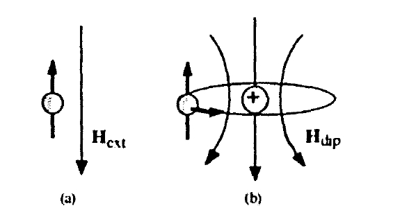
Figure 2.4. Spin magnetism: (a) Zeeman interaction and (b) spin-orbit coupling.
is known as the one-electron spin-orbit coupling constant. For hydrogen-like atoms this equation reduces to
\(\lambda = \frac{m_{e} c^{4}}{2} \frac{Z^{4}}{n^{3}l(l + 1/2)(l + 1)}\). (2.39)
Typical orders of magnitude of \(\lambda\), measured in kelvin, are 500 K for iron-series 3d electrons and 2000 K for rare-earth 4f electrons. It is worth mentioning that the \(\hat{l} \cdot \hat{s}\) form of the spin-orbit coupling is restricted to spherical potentials. In general, this term is proportional to \((\hat{s} \times \nabla\varphi_{e}) \cdot \hat{p}\), indicating that the spin-orbit coupling requires the motion of the electrons to be perpendicular to both the spin moment and the electrostatic field \(\nabla\varphi_{e}\).
Spin-orbit coupling is of central importance in permanent magnetism, which requires the spins to be coupled to the motion of the electrons in an anisotropic crystal environment (section 3.1). It is usually the main source of magnetocrystalline anisotropy.
Magnetic Forces and susceptibilities: How They Work
Magnetostatic Interactions with External Fields
In terms of microscopic averages \(\langle m \rangle = \langle \hat{m} \rangle\), the Zeeman energy appearing in the Pauli equation is given by (1.11) and (1.12). More generally,
\(E_{Z} = -\mu_{0} \int M(r) \cdot H(r) dr\). (2.40)
The Zeeman energy determines the interaction of a permanent magnet with external magnetic fields. For example, in a weakly inhomogeneous magnetic field \(H(r) = H(r_{0}) + (r - r_{0}) \cdot \nabla H\), the force \(F = -\partial E_{Z} / \partial r\) acting on a permanent magnetic dipole is given by (1.12), which can be rewritten as
\(F_{i} = \mu_{0}m \cdot \frac{\partial H}{\partial x_{i}}\). (2.41)
This equation applies to paramagnetic dipoles as well, since the interaction of a moment with a field does not depend on the sample's past. If it is possible to write \(m = \chi H\Omega\), where \(\chi\) is the paramagnetic susceptibility, then (2.41) becomes3
\(F = \frac{\mu_{0}\chi\Omega}{2} \nabla(H^{2})\). (2.42)
This equation predicts that the force diverges in the limit of very soft materials, where \(\chi = \partial M / \partial H\) is very large. In fact, soft magnetic materials saturate in very small fields, so that (2.41) is the relevant equation. Only materials which do not saturate in the applied field can be described by (2.42).
To derive the torque acting on a magnetic dipole it is sufficient to rewrite the Zeeman energy as \(E_{Z} = -\mu_{0}mH \cos\theta\), where \(\theta\) is the angle between field and moment. Taking the derivative with respect to \(\theta\) then yields \(\Gamma = \mu_{0}mH \sin\theta\) (1.13).
Susceptibilities
Equations of state and magnetization curves are obtained by minimizing the total magnetic energy with respect to \(M(r)\). However, the magnetic energy contains not only the Zeeman term but also other energy contributions such as exchange, anisotropy and magnetostatic self-interaction. A qualitative method of analysing the strengths of magnetic interactions is susceptibility analysis.
In a general sense, susceptibility is defined as \(\chi = \partial M / \partial H\) and describes the response of the magnetization to a small change in the external field. External fields always tend to increase the magnitude of the magnetization, but the Zeeman interaction has to compete against other energy contributions (table 2.1). Usually the magnetostatic self-interaction of ferromagnets is excluded from this consideration, since it yields low-field susceptibilities which depend on the sample's history.
High-field susceptibilities indicate to what extent the Zeeman interaction is able to compete against the effect of (electronic) electrostatic interactions. From the relativistic nature of magnetic interactions (section 2.1.3), it follows that high-field susceptibilities are of the order of \(\alpha^{2}\), so that fields of more than 100 T are needed to produce a polarization of 0.01 T. Depending on whether the sum of all susceptibility contributions is positive or negative, a material is called a paramagnet or a diamagnet. Typical susceptibilities are \(0.08\times 10^{-4}\) for Na, \(0.21\times 10^{-4}\) for Al, \(-0.10\times 10^{-4}\) for Cu and \(-0.12\times 10^{-4}\) for NaCl. The paramagnetism of simple metals, referred to as Pauli paramagnetism (section 2.4.1.2), is nearly temperature independent (figure 2.5(a)). Pauli paramagnetism has to be contrasted with the strongly temperature-dependent Curie-Langevin paramagnetism (section 2.3), which reflects the competition
3 In this chapter we use the symbol \(\Omega\) to denote the magnet's volume, to avoid confusion with electrostatic potentials.
Table 2.1.Typical susceptibilities. All temperatures and energies are measured in kelvin.
| Type | Order of magnitude | Example | Basic feature |
|---|---|---|---|
| Zeeman interaction versus electrostatic interaction | |||
| Pauli paramagnetism | +\(\alpha^{2}\) | Na | Splitting of Fermi level |
| Atomic diamagnetism | -\(\alpha^{2}\) | NaCl | Induction (Lenz's law) |
| Landau diamagnetism | -\(\alpha^{2}\) | Cu | Induction (Lenz's law) |
| Zeeman interaction supported by electrostatic interaction | 1/\(T^{3}\) | Gd\(_2\)O\(_3\) | Thermal disorder |
| Van Vleck paramagnetism | 1/\(\Delta E\) | Eu\(_2\)O\(_3\) | Higher multiplets |
| Enhanced Pauli paramagnetism | \(\chi \gg \alpha^{2}\) | Pd | Splitting of Fermi level |
| Diamagnetism of superconductors | -1 | Pb | Induction (Lenz's law) |
| Curie-Weiss paramagnetism (above \(T_C\)) | 1/(\(T - T_C\)) | Gd | Thermal disorder and exchange |
| Ferromagnetic susceptibilities in metals | \(\geq 1\) | Fe | Involves magnetic fields and anisotropyc |
| High-field susceptibility | \(\alpha^{2}\) | Fe | Electronic originc |
a Also known as Langevin paramagnetism.
b These approximate relations, where \(T\) is measured in kelvin, derive from the temperature equivalent \(0.672 \text{ K}^{-1}\), where \(T\) is the Bohr magneton and reflect the fundamental fact that atomic magnetic moments and atomic lengths are of order \(\mu_B\) and \(\text{A}\), respectively.
c History dependent.
d Equivalent to Pauli paramagnetism.
between the Zeeman interaction and thermal disorder and obeys the Curie law \(\chi = C/T\) (figure 2.5(b)). For materials with \(\mu_{0}M_{0} \approx 1 \text{ T}\), the order of magnitude of the Curie constant \(C\) is epitomized by the ratio of the Bohr magneton to Boltzmann's constant \(\mu_{B}/k_{B} = 0.672 \text{ K}^{-1}\). Low-temperature thermal excitations are therefore very effective in overcoming the spin alignment in external fields, and typical magnetostatic fields of order \(1 \text{ T}\) are quite unable to produce room-temperature ferromagnetic order. For this reason some stronger coupling mechanism, namely the electrostatic exchange interaction, is required to explain room-temperature ferromagnetism. In other words, the onset of ferromagnetism—defined by the existence of a spontaneous magnetization in zero field—is accompanied by a Curie-Weiss susceptibility which diverges at the Curie temperature due to strong exchange interactions.
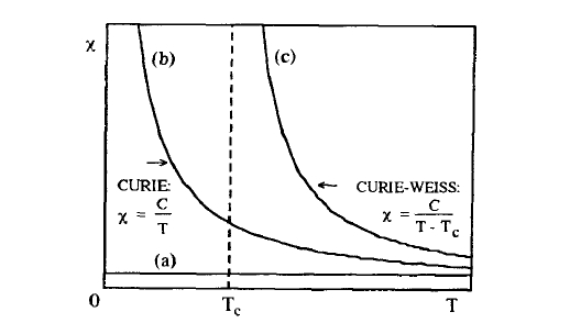
Figure 2.5. Schematic temperature dependence of magnetic susceptibilities: (a) Pauli paramagnetism, (b) Curie–Langevin paramagnetism and (c) Curie–Weiss paramagnetism of a ferromagnet above \(T_{C}\).
Diatomic Two-Electron Exchange: A Deeper Look
So far, we have focused on the behaviour of isolated electrons in external magnetic and electric fields. External magnetic fields are able to fix the moment parallel to the field direction, but the question remains of how ferromagnetic order is realized in the absence of magnetic fields of more than 100 T. One candidate is the mutual dipolar interaction of the electrons in the solid, but we have just seen that the smallness of the Zeeman interaction leads to the destruction of magnetostatic order above temperatures of order 1 K. In fact, as shown by Heisenberg (1928) and Bloch (1929), ferromagnetic coupling is essentially electrostatic caused by the exchange interaction.
There are two types of exchange: intra-atomic exchange responsible for the formation of atomic magnetic moments and inter-atomic exchange responsible for magnetic order. Here we consider inter-atomic two-electron exchange in a diatomic model and focus on the Heisenberg model and the Hartree–Fock approximation. Hund's intra-atomic exchange will be treated in section 2.2, whereas Heisenberg interactions in real materials and itinerant exchange will be dealt with in section 2.3 and section 2.4, respectively.
Exchange As A Many-body Problem
Exchange derives from the many-electron Schrödinger equation (2.13), but the intractability of that equation leads us to the consideration of the two-electron Schrödinger equation as a starting point. Note that the two-electron problem contains much of the essential physics of the many-electron problem, and quantities such as the Coulomb repulsion \(U\) of two electrons on the same site, the transfer or hopping integral \(T\) giving the bandwidth, and the direct exchange \(J_D\)
all appear in embryo in the two-electron system. The two-electron Schrödinger equation can be written as
\(E\Psi = -\frac{\hbar^{2}}{2m} \frac{\partial^{2}\Psi}{\partial r^{2}} - \frac{\hbar^{2}}{2m} \frac{\partial^{2}\Psi}{\partial r'^{2}} + V_{0}(r)\Psi + V_{0}(r')\Psi + V_{c}(r, r')\Psi\). (2.43)
Here \(r\) and \(r'\) are the positions of the two electrons, respectively, \(V_{c} = e^{2}/4\pi\epsilon_{0}|r - r'|\) and \(V_{0}\) is the potential in the vicinity of two neighbouring atoms. Note that there is no explicit spin dependence in (2.43) – the magnetic character of the solutions of that equation is hidden in the two-electron wavefunctions \(\Psi(r, r')\). For instance, a solution where both electrons are located at the same orbital must have an antiparallel spin structure, \(\downarrow\uparrow\) when there is no orbital degeneracy, since the Pauli principle forbids \(\uparrow\uparrow\) and \(\downarrow\downarrow\) occupancies of a given orbital.
One-electron States
Consider a symmetric one-electron potential \(V_{0}(r) = V_{at}(|r|) + V_{at}(|r - R|)\), where \(V_{at}\) may be interpreted as an atomic potential and \(R\) is the inter-atomic distance. Let us, for the moment, neglect the Coulomb repulsion \(e^{2}/(4\pi\epsilon_{0}|r - r'|)\), so that (2.43) reduces to \(\Psi(r, r') = \phi(r)\phi(r')\) and
\(E\phi = -\frac{\hbar^{2}}{2m} \frac{\partial^{2}\phi}{\partial r^{2}} + V_{at}(r)\phi + V_{at}(r - R)\phi\). (2.44)
The energies of the ground and first excited states are \(E_{0} - \Delta E_{0}\) and \(E_{0} + \Delta E_{0}\), respectively. Essentially, the hybridization energy \(\Delta E_{0} \approx -T_{0}\) is given by the hopping integral
\(T_{0} = \int \phi_{at}(r)V_{at}(r)\phi_{at}(r - R) dr\) (2.45)
calculated from atomic wavefunctions \(\phi_{at}\). Note that hopping integrals approach zero in the limit of infinite separation \(R\).
Figure 2.6 shows that the ground-state wavefunction \(\phi_{S}\) is symmetric, whereas the wavefunction \(\phi_{A}\) of the first excited state is antisymmetric. A way of rationalizing the symmetry of the one-electron wavefunctions is to think of \(\phi_{S}\) and \(\phi_{A}\) as rudimentary Bloch wavefunctions having \(k = 0\) and \(k = \pi/R\), respectively. In this sense, \(\phi_{S}\) and \(\phi_{A}\) are delocalized, that is metallic, and \(2T_{0}\) is a rudimentary bandwidth.
In the present context it is useful to replace \(\phi_{S}\) and \(\phi_{A}\) by localized Wannier functions (figure 2.7)
\(\phi_{L} = \frac{1}{\sqrt{2}}(\phi_{S} + \phi_{A})\) and \(\phi_{R} = \frac{1}{\sqrt{2}}(\phi_{S} - \phi_{A})\). (2.46)
4 Atomic wavefunctions are non-orthogonal, so that the relation \(\Delta E_{0} = -T_{0}\) is only approximate. One example where the energy splitting is known exactly is the \(H_{2}^{+}\) ion.
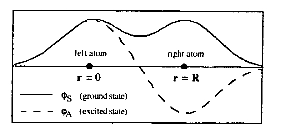
Figure 2.6. Diatomic exchange model: schematic one-electron wavefunctions.
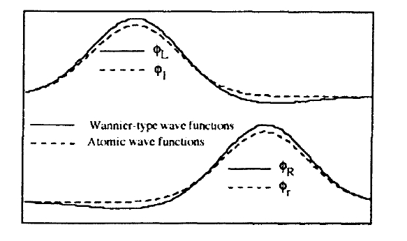
Figure 2.7. Wannier functions and true atomic wavefunctions (schematic).
The relation \(\int \phi_{S}(r)\phi_{A}(r) dr = 0\) implies \(\int \phi_{L}(r)\phi_{R}(r) dr = 0\), so that both sets of wavefunctions are orthogonal. Equation (2.46) is easily inverted to reproduce the delocalized wavefunctions
\(\phi_{S} = \frac{1}{\sqrt{2}}(\phi_{L} + \phi_{R})\) and \(\phi_{A} = \frac{1}{\sqrt{2}}(\phi_{L} - \phi_{R})\). (2.47)
The localized wavefunctions \(\phi_{L}\) and \(\phi_{R}\) are reminiscent of, but not equivalent to, the atomic orbitals \(\phi_{l}(r) = \phi_{at}(r)\) and \(\phi_{r}(r) = \phi_{at}(r - R)\) (figure 2.7). This is seen, for example, from the non-orthogonality of \(\phi_{l}\) and \(\phi_{r}\). In the present model, the relation between the two sets of wavefunctions is
\(\phi_{L/R} = \frac{1}{2}\left(\frac{1}{\sqrt{1 - S}} + \frac{1}{\sqrt{1 + S}}\right)\phi_{l/r} - \frac{1}{2}\left(\frac{1}{\sqrt{1 - S}} - \frac{1}{\sqrt{1 + S}}\right)\phi_{r/l}\) (2.48)
where \(S\) is the orthogonality integral \(\int \phi_{r}^{*}(r)\phi_{l}(r) dr\). It is worth emphasizing that neither \(\phi_{L}\) and \(\phi_{R}\) nor \(\phi_{l}\) and \(\phi_{r}\) are eigenfunctions of the one-electron problem; the only advantage of these sets of wavefunctions is that they are localized in real space rather than in \(k\) space.
Two-electron Wavefunctions
Having selected a convenient set of orthogonal one-electron wavefunctions—let us choose \(\phi_{l}\) and \(\phi_{R}\)—we can construct two-electron wavefunctions. There are four possible ways of forming product functions \(\Psi_{i} = \Psi_{i}(r, r')\) from \(\phi_{l}\) and \(\phi_{R}\): \(\Psi_{1} = \phi_{l}(r)\phi_{l}(r')\), \(\Psi_{2} = \phi_{l}(r)\phi_{R}(r')\), \(\Psi_{3} = \phi_{R}(r)\phi_{l}(r')\) and \(\Psi_{4} = \phi_{R}(r)\phi_{R}(r')\). These four orthogonal two-electron wavefunctions form a complete set so long as only the two lowest-lying one-electron states are considered.
The eigenfunctions and eigenvalues of the two-electron problem (2.43) are now obtained by diagonalizing the interaction matrix
\(E_{ik} = \int \Psi_{i}^{*}(r, r')\mathcal{H}\Psi_{k}(r, r') dr dr'\).
Up to a physically irrelevant zero-point energy, the interaction matrix is
\(E_{ik} = \begin{pmatrix} U & \mathcal{T} & \mathcal{T} & \mathcal{J}_{D} \\ \mathcal{T} & 0 & \mathcal{J}_{D} & \mathcal{T} \\ \mathcal{T} & \mathcal{J}_{D} & 0 & \mathcal{T} \\ \mathcal{J}_{D} & \mathcal{T} & \mathcal{T} & U \end{pmatrix}\). (2.49)
Here the hopping integral \(\mathcal{T} = -\Delta E\) differs from \(T_{0}\) by minor two-electron corrections. It may be interpreted as half the bandwidth, which is a few eV in transition metals. Apart from minor corrections, the Coulomb interaction parameter equals the electrostatic energy necessary to add a second electron into a localized orbital
\(U = \int \phi_{L}(r)\phi_{L}(r')V_{c}(r - r')\phi_{L}(r')\phi_{L}(r) dr dr'\). (2.50a)
Since two atoms in one atomic orbital feel a strong electrostatic repulsion, \(U\) is large and positive, typically a few eV. The direct exchange
\(\mathcal{J}_{D} = \int \phi_{l}(r)\phi_{R}(r')V_{c}(r - r')\phi_{l}(r')\phi_{R}(r') dV dV'\) (2.50b)
is also positive, but for inter-atomic distances of interest it is no larger than about 0.1 eV, that is it is smaller than \(U\) and \(\Delta E\) by at least one order of magnitude. Note, furthermore, that both \(J_{D}\) and \(\Delta E\) decrease exponentially with increasing inter-atomic distance and are negligibly small for \(R \gg 1 \text{ A}\).
A nice feature of the two-electron problem is the fact that the interaction matrix (2.49) can be diagonalized analytically. The first eigenstate is characterized by the energy \(U - \mathcal{J}_{D}\) and the wavefunction \([\phi_{l}(r)\phi_{l}(r') + \phi_{R}(r)\phi_{R}(r')]/\sqrt{2}\). Since \(U\) is large and positive, this state is of no interest in the present context. The same refers to the second state, whose energy is even higher than \(U\). The third eigenfunction
\(\Psi_{\text{FM}} = \frac{1}{\sqrt{2}}[\phi_{l}(r)\phi_{R}(r') - \phi_{R}(r)\phi_{l}(r')]\) (2.51)
corresponds to a delocalized ferromagnetic state of energy \(E_{\text{FM}} = -\mathcal{J}_{D}\), and the fourth eigenfunction is
\(\Psi_{\text{AFM}} = \frac{\sin \chi}{\sqrt{2}}[\phi_{l}(r)\phi_{l}(r') + \phi_{R}(r)\phi_{R}(r')] + \frac{\cos \chi}{\sqrt{2}}[\phi_{l}(r)\phi_{R}(r') + \phi_{R}(r)\phi_{l}(r')]\) (2.52)
where \(\tan(2\chi) = 4\Delta E / U\). This means that the inter-atomic hopping \((\Delta E)\) leads to an electrostatically unfavourable admixture of double-occupied states \((\chi \neq 0)\). The energy associated with (2.52) is
\(E_{\text{AFM}} = \frac{U}{2} + \mathcal{J}_{D} - \sqrt{4\Delta E^{2} + \frac{U^{2}}{4}}\). (2.53)
To interpret these eigenvalues and eigenfunctions we need to know the spin alignment of the two electrons.
Spin Structure
In the diatomic two-electron model, parallel \((\uparrow\uparrow)\) and antiparallel \((\uparrow\downarrow)\) spin orientations mean ferromagnetism and antiferromagnetism (or a covalent bond), respectively. A simple way to decide whether the spin orientation is ferromagnetic or antiferromagnetic is to investigate the symmetry of the orbital wavefunctions. Symmetric wavefunctions, \(\Psi(r, r') = \Psi(r', r)\), give rise to antiferromagnetism, whereas antisymmetric wavefunctions, characterized by \(\Psi(r, r') = -\Psi(r', r)\), yield ferromagnetic order. This rule is linked to the Pauli principle, which forbids \(\uparrow\uparrow\) and \(\downarrow\downarrow\) occupancies of a single orbital. Note that a more detailed derivation of the rule is based on the consideration of wavefunctions which are both space and spin dependent. The ferromagnetic state \(\Psi_{F}\) then forms a Zeeman triplet \((m_{S} = 1)\), \(\uparrow\uparrow (m_{S} = 0)\) and \(\downarrow\downarrow (m_{S} = -1)\).
It is convenient to define an effective exchange constant
\(\mathcal{J}_{\text{eff}} = \frac{1}{2}(E_{\text{AFM}} - E_{\text{FM}})\) (2.54)
so that
\(\mathcal{J}_{\text{eff}} = \mathcal{J}_{D} + \frac{U}{4} - \sqrt{\Delta E^{2} + \frac{U^{2}}{16}}\). (2.55)
In this equation, \(\mathcal{J}_{\text{eff}} > 0\) indicates ferromagnetism, as this minimizes the energy.
From (2.55) we see that inter-atomic hopping \(T = -\Delta E\) tends to destroy ferromagnetism. The competition between one-electron energies, epitomized by \(\Delta E\), and two-electron interactions is illustrated in table 2.2. Strong inter-atomic hopping leads to a large energy splitting \(\pm\Delta E\) of the one-electron levels, which makes the ferromagnetic state energetically unfavourable compared to the antiferromagnetic configuration. On the other hand, the Coulomb term \(V_{2}\) favours ferromagnetism: \(\uparrow\downarrow\) electron pairs in a localized orbital have high electrostatic energies, whereas \(\uparrow\uparrow\) pairs in a single orbital are forbidden by the Pauli principle.
Table 2.2. Atomic origin of ferromagnetism. The double arrow (\(\Leftrightarrow\)) indicates some degree of mixing in the antiferromagnetic case, corresponding to (2.52).
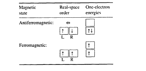
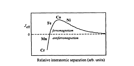
Figure 2.8. The Bethe-Slater-Neel curve.
The Bethe–Slater– Néel Curve
Since the Curie temperature increases with \(J_{\text{eff}}\), it is instructive to compare (2.55) with the semiphenomenological Bethe–Slater– Néel curve shown in figure 2.85. The curve predicts antiferromagnetism in the case of small inter-atomic distances, ferromagnetism at intermediate distances and the absence of magnetic order in the limit of very large inter-atomic distances. This general trend is indeed observed in iron and many iron-rich alloys, but it is difficult to relate the curve to the detailed electronic structure. Equation (2.50) shows that the direct exchange \(J_{D}\) increases with decreasing inter-atomic distance, so that \(J_{D}\) cannot be responsible for the short-distance breakdown of ferromagnetism shown in
5 Depending on whether the argument is the inter-atomic distance divided by the 3d shell radius (as in Sommerfeld and Bethe 1933) or for example the distance between the magnetic shells, there are different variants of this curve.
figure 2.8. Furthermore, metallic moments and Curie temperatures do not depend on the inter-atomic distances only but also depend on factors such as the crystal structure and band filling (section 2.4.3), so that the Bethe–Slater– Néel curve is at best qualitative (see also section 2.3.1.4).
Many-Body Models and Approximations in Magnetism
The diagonalization of the two-electron matrix (2.49) is one of the few quantum-mechanical many-body problems which can be solved exactly. In practice, ferromagnetism is a fairly intractable multi-atom and multi-electron problem, and there are no simple rules to predict the outcome of the competition between interaction terms and one-electron energies in real solids. The hydrogen molecule turns out to be antiferromagnetic at all inter-atomic distances, which is known as the Lieb–Mattis theorem, but in some oxides and in many metals the coupling is ferromagnetic. The main reason is the involvement of atomic d or f orbitals, which not only feel a local potential as in (2.43) but are also orthogonal to the core wavefunctions. However, to discuss the main features of many-body approximations such as the Hartree–Fock theory and the Heisenberg model we can restrict ourselves to the two-electron model.
One-electron Approximation
Hartree–Fock wavefunctions are Slater determinants composed of suitable one-electron wavefunctions. A simple example of a Slater determinant is the wavefunction \(\psi_{B}(r)\psi_{C}(r') - \psi_{C}(r)\psi_{B}(r')\), which describes two electrons in the states B and C, respectively. Hartree–Fock wavefunctions obey the Pauli principle and contain many-body interactions in an approximate form. Many-body effects going beyond the Hartree–Fock approximation are known as correlation effects.
The determination of optimum one-electron wavefunctions is a complicated problem and in practice one has to use approximations such as local-density theory. A very crude approach is to use unperturbed eigenfunctions. For example, using (2.46) and (2.51) we can rewrite the ferromagnetic wavefunction as
\(\Psi_{\text{FM}}(r, r') = \frac{1}{\sqrt{2}}(\phi_{S}(r)\phi_{A}(r') - \phi_{A}(r)\phi_{S}(r'))\) (2.56)
and reproduce \(E_{\text{FM}} = -\mathcal{J}_{D}\). This equation means that one \(\uparrow\) electron is in the ground state and one \(\uparrow\) electron is in the first excited state. The antiferromagnetic Hartree–Fock state is obtained by accommodating two electrons of opposite spin in the one-electron ground state. This yields the ground-state energy \(U/2 - 2\Delta E + \mathcal{J}_{D}\), so that
\(\mathcal{J}_{\text{HF}} = \mathcal{J}_{D} + \frac{U}{4} - \Delta E\). (2.57)
The same result is obtained by putting \(\Delta E \gg U\) in (2.55).
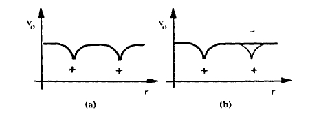
Figure 2.9. Effective one-electron potentials ( schematic ): ( a ) symmetric potential and (b) unrestricted Hartree-Fock potential whose symmetry is reduced by screening (aside from secondary crystal - field affects, the one -electron wave functions are atomic ).
From (2.57) we can draw a number of important conclusions. First, the Hartree–Fock approximation is exact in the limit \(\Delta E \gg U\), that is in the itinerant limit of strong inter-atomic hopping. Second, ferromagnetism is predicted in narrow bands whose width \(W = -2\Delta E\) obeys
\(W \leq \frac{U}{2} + 2\mathcal{J}_{D}\). (2.58)
Generalized to real metals, this condition is known as the Stoner criterion and gives a reasonable description of itinerant ferromagnets such as elemental iron, YFe2 and Y2Fe14B (section 2.4).
Comparing (2.55) and (2.57) we see that the Hartree–Fock approximation overestimates the tendency towards ferromagnetism. In fact, since \(\Delta E\) and \(\mathcal{J}\) vanish for well separated atoms but \(U\) remains finite, it leads to the physically unreasonable prediction of strong ferromagnetic coupling between isolated electrons. The reason for this failure is the neglect of localized states in the Hartree–Fock approximation. Figure 2.9(a) shows a typical one-electron potential leading to Bloch-symmetric one-electron wavefunctions such as those shown in figure 2.6. In fact, the symmetry of the one-electron potential is reduced by Coulomb repulsion which suppresses double occupancy of localized orbitals (figure 2.9(b)). This correlation is particularly strong in narrow bands where inter-atomic hopping is not able to remove electrons from localized states.
Hubbard Model
A particular model which aims at interpolating between the localized and delocalized limits by neglecting the direct exchange is the Hubbard model. In terms of the matrix (2.49) it is defined by \(\mathcal{J}_{D} = 0\), but it can also be written as \(\mathcal{H} = \hat{i} + U\hat{n}_{\uparrow}\hat{n}_{\downarrow}\), where \(\hat{i}\) is a one-electron hopping operator and the \(\hat{n}_{\sigma}\) are spin-dependent fermionic particle-number operators (see also sections 2.4.2.2
Putting \(U \gg \Delta E\) in (2.55) yields the so-called kinetic exchange6
\(\mathcal{J}_{\text{eff}} = -\frac{2\Delta E^{2}}{U}\). (2.59)
This exchange contribution, which is not restricted to the two-electron problem, is antiferromagnetic and reflects the destruction of ferromagnetic coupling by inter-atomic hopping. The Hubbard model not only reproduces the observed vanishing of \(\mathcal{J}_{\text{eff}}\) in the limit of infinite inter-atomic separation, but also describes the transition from metallic to non-metallic behaviour beyond some critical inter-atomic spacing. Electron localization due to many-body interactions is referred to as Mott localization, as opposed to Anderson localization caused by intrinsic lattice disorder.
Heisenberg Model
Heisenberg (1928) used the Heitler–London approximation to explain ferro- and antiferromagnetism in terms of direct exchange between localized electrons. Heisenberg's starting point is electrons localized in atomic orbitals \(\phi_{l}\) and \(\phi_{r}\), from which wavefunctions \(\phi_{l}(r)\phi_{r}(r') \pm \phi_{r}(r)\phi_{l}(r')\) are constructed. The Heisenberg exchange constant \(J_{\text{He}}\) therefore contains the orthogonality integral \(S\) (section 2.1.5.2). In the limit \(U \gg \Delta E\), both (2.55) and the Heisenberg model yield
\(\mathcal{J}_{\text{eff}} = \mathcal{J}_{D} - \frac{2\Delta E^{2}}{U}\). (2.60)
Unfortunately, slight modifications of the localized one-electron wavefunctions used to construct the two-electron states alter the predictions of the Heisenberg model quite drastically. For example, replacing the atomic wavefunctions \(\phi_{l}\) and \(\phi_{r}\) by Wannier functions \(\Phi_{l}\) and \(\Phi_{r}\) leads to \(\mathcal{J}_{\text{eff}} = \mathcal{J}_{D}\). The reason is that \(f \int \Phi_{l}(r)\Phi_{r}(r) dr = 0\), whereas the original Heisenberg model needs some overlap to realize the kinetic exchange contribution. This difficulty is even more pronounced if more than two electrons are considered, and in the solid-state limit the use of non-orthogonal wavefunctions leads to divergent many-electron corrections referred to as the non-orthogonality catastrophe (Slater 1953).
In practice, the Heisenberg model works reasonably well for local-moment ferromagnets such as EuO and Gd. Although it is possible to derive expressions such as (2.60) perturbatively from many-body equations, it is common to treat the Heisenberg model as a phenomenological parameter. The two-spin Heisenberg model is then easily generalized to solids. Since \((\vec{s}_{1} + \vec{s}_{2})^{2} = s_{1}^{2} + s_{2}^{2} + 2\vec{s}_{1} \cdot \vec{s}_{2}\) and
6 See, for example, Anderson (1963), Goodenough (1963) and Jones and March (1973).
\(\langle\vec{s}^{2}\rangle = \hbar^{2}s(s + 1)\), the exchange splitting \(\pm\mathcal{J}_{\text{eff}}\) is reproduced by the spin Hamiltonian
\(\mathcal{H} = -\frac{2\mathcal{J}_{\text{eff}}}{\hbar^{2}}\vec{s}_{1} \cdot \vec{s}_{2}\). (2.61)
Here \(\vec{s}_{1}\) and \(\vec{s}_{2}\) can be interpreted as real-space vectors whose scalar product indicates parallel or antiparallel spin alignment. In the solid-state limit, we have the Heisenberg Hamiltonian
\(\mathcal{H} = -\frac{2}{\hbar^{2}}\sum_{i < k}J_{ik}\vec{S}_{i} \cdot \vec{S}_{k} - \frac{2\mu_{B}\mu_{0}}{\hbar}\sum_{i}\boldsymbol{H}_{i} \cdot \vec{S}_{i}\) (2.62)
where the phenomenological exchange constants \(J_{ik}\) describe the exchange coupling between atomic spins \(\vec{S}_{i}\) and \(\vec{S}_{k}\) located at \(r_{i}\) and \(r_{k}\), respectively. Subject to some refinements (section 2.3), the Heisenberg model is a widely used approach which parametrizes exchange in terms of a few exchange constants.
Validity of The Two-Electron Model
Summarizing, the diatomic two-electron model gives a qualitatively correct description of inter-atomic exchange. The delocalized Hartree–Fock limit applies to itinerant magnetism, whereas the Heisenberg limit describes the coupling between local moments. However, even itinerant 3d electrons retain some localized character by forming virtual bound states, which affect both anisotropy and Curie temperature (sections 2.4 and 3.1).
The antiferromagnetism of the simplest realization of the diatomic two-electron model (the H2 molecule) is another shortcoming. First, in general there are more than one or two magnetic electrons per atom, which gives rise to intra-atomic exchange between electrons in the different orbitals. Since one-electron energy splittings are smallest for nearly degenerate atomic levels, moment formation is easy for electrons in partly filled d and f shells. Second, the two-electron model neglects the presence of other classes of electrons, such as oxygen valence electrons in oxides or 4s conduction electrons in iron-series transition metals and alloys. In spite of their small spin polarization, these electrons affect the magnetic properties, for example by giving rise to the important indirect exchange in metals (section 2.3.1) or superexchange in oxides.
Magnetostatic Interactions: The Forces Between Magnetic Materials
Besides the Zeeman interaction between electrons and the external magnetic field there exist magnetostatic self-interactions between the atomic moments of a magnet. We have seen that magnetostatic many-body interactions are much weaker than exchange interactions, but equations such as (2.8) show that they are long ranged, as opposed to the essentially short-ranged exchange interaction. For this reason, magnetostatic interactions are negligible on an atomic scale yet dominate macroscopic magnetism. In this subsection, we discuss magnetostatic
fields and interactions associated with a given magnetization \(M(r)\); the dependence of \(M(r)\) on magnetostatic fields is dealt with in chapter 3.
Magnetostatic Energy
Equation (2.40) gives the magnetostatic energy of a dipole \(m_{j}\) in an external magnetic field. From a basic point of view, there is no difference between an external field and the field \(H_{j}\) caused by another atomic dipole \(m_{i}\), and the interaction energy between two dipoles \(m_{i}\) and \(m_{j}\) is
\(E^{*} = -\mu_{0}H_{i} \cdot m_{j} = -\mu_{0}H_{j} \cdot m_{i}\). (2.63)
Adding the contributions of all atomic pairs yields
\(E^{*} = -\frac{\mu_{0}}{2} \sum_{i,j} m_{i} \cdot H_{j}\) (2.64)
where the factor \(1/2\) is necessary because the sum contains each pair twice.
Apart from a constant term, \(E^{*}\) equals the magnetostatic self-energy \(E_{\text{ms}} = -(\mu_{0}/2) \int M \cdot H_{\text{dm}} \text{d}V\) introduced in section 1.1.1.4. Here we will start with the continuum interpretation of magnetostatics, which involves the demagnetizing dipole field \(H_{\text{dm}}\) introduced in section 1.1.1.
Demagnetizing Fields
A straightforward way of determining the demagnetizing field \(H_{\text{dm}}\) acting in a magnet is to solve the magnetostatic Maxwell equations. In uniformly magnetized ellipsoids the calculation yields a dipolar field which is homogeneous throughout the magnet7, and when the field is applied along a principal axis then \(H_{\text{dm}}\) is given by (1.9). Otherwise,
\(\begin{pmatrix} H_{x}^{\text{dm}} \\ H_{y}^{\text{dm}} \\ H_{z}^{\text{dm}} \end{pmatrix} = -\begin{pmatrix} D_{xx} & D_{xy} & D_{xz} \\ D_{yx} & D_{yy} & D_{yz} \\ D_{zx} & D_{zy} & D_{zz} \end{pmatrix} \begin{pmatrix} M_{x} \\ M_{y} \\ M_{z} \end{pmatrix}\). (2.65)
Here the matrix elements \(D_{kl}\) are the demagnetizing factors and the negative sign indicates that \(M\) and \(H_{\text{dm}}\) point in opposite directions. From the dipolar character of the magnetostatic interaction, it follows that the trace of the demagnetizing tensor is equal to one.
In ellipsoids of revolution the rotational symmetry leads to the principal-axis representation
\(\begin{pmatrix} H_{x}^{\text{dm}} \\ H_{y}^{\text{dm}} \\ H_{z}^{\text{dm}} \end{pmatrix} = -\begin{pmatrix} D_{\perp} & 0 & 0 \\ 0 & D_{\perp} & 0 \\ 0 & 0 & D_{\parallel} \end{pmatrix} \begin{pmatrix} M_{x} \\ M_{y} \\ M_{z} \end{pmatrix}\) (2.66)
7 Dipole fields in free space and in non-ellipsoidal magnets tend to be inhomogeneous.
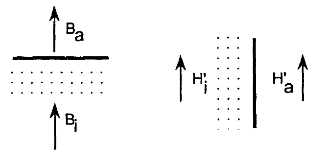
Figure 2.10. Magnetic fields at phase boundaries.
where \(2D_{\perp}+D_{\parallel}=1\) and, in standard notation, \(D_{\parallel}=D\) and \(D_{\perp}=(1 - D)/2\). If \(M\) and \(H\) are parallel to the axis of revolution \((e_{z})\) then the total field is given by the expression
\(H' = H - DM\). (2.67)
To calculate \(D\) one can use the integral representation (2.5) of the magnetostatic equations. A consequence of those equations is that the perpendicular component of \(B\) as well as the parallel component of \(H'\) remain continuous at phase boundaries (figures 1.2 and 2.10). Using the indices \(i\) and \(a\) to denote fields inside and outside the magnet, respectively, we obtain from (1.4) the boundary conditions \(H_{a}'(\perp)=H_{i}'(\perp)+M(\perp)\) and \(H_{a}'(\parallel)=H_{i}'(\parallel)\). Let us first determine \(D\) for spherical \((R_{x}=R_{y}=R_{z})\), prolate \((R_{z}>R_{x}=R_{y})\) and oblate \((R_{z} Spheres do not have special surface directions, so it is necessary to incorporate both boundary conditions. In free space, the dipole field created by the sphere is \(2M_{s}e_{z}/3\) and \(-M_{s}e_{z}/3\) at the surface points III and IV, respectively. At both points the boundary conditions yield \(H_{i}'=H_{a}'-M_{s}/3\), so that \(D = 1/3\). An easier way to derive this demagnetizing factor is to use Trace \(D_{ik}=1\), which means that \(D = 1/3\) by symmetry. Demagnetizing factors for prolate and oblate ellipsoids with intermediate aspect ratios \(\kappa_{0}=R_{z}/R_{x}\) are (Osborn 1945) \(D=\frac{1}{\kappa_{0}^{2}-1}\left(\frac{\kappa_{0}}{\sqrt{\kappa_{0}^{2}-1}}\text{arcosh}\kappa_{0}-1\right)\) (2.68a)
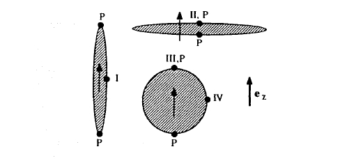
Figure 2.11. Calculation of demagnetizing fields in ellipsoids of revolution. The arrow shows the common magnetization direction of the three magnets. The meaning of the symbols is explained in the main text.
and
\(D = \frac{1}{1-\kappa_{0}^{2}}\left(1-\frac{\kappa_{0}}{\sqrt{1-\kappa_{0}^{2}}}\text{arccos}\kappa_{0}\right)\) (2.68b)
respectively. As discussed above, spherical particles exhibit \(\kappa_{0} = 1\) and \(D = 1/3\). In the limits of needle-shaped \((\kappa_{0} \gg 1)\) and plate-like \((\kappa_{0} \ll 1)\) magnets, (2.68) reduces to
\(D = \frac{1}{\kappa_{0}^{2}}(\ln\kappa_{0} - 0.307)\) and \(D = 1-\frac{\pi}{2}\kappa_{0}\) (2.69)
respectively. Table 2.3 gives numerical values calculated from (2.68).
It is worth noting that the validity of (2.68) is limited to ellipsoidal magnets. For cylinders one obtains, for example, volume-averaged demagnetizing factors \(D(L/2R)\): \(D(0.5) = 0.4645\), \(D(1) = 0.3116\), and \(D(2) = 0.1819\), but the demagnetizing field is not quite uniform throughout the body of the magnet.
Another configuration where the demagnetizing field can be calculated in a closed form is in toroidal magnets with small air gaps (figure 2.12). The equation \(\int \boldsymbol{B} \cdot d\boldsymbol{S} = 0\) then reduces to \(H_{g} = H_{m} + M\), and \(\oint \boldsymbol{H} \cdot d\boldsymbol{l} = 0\) yields \(l_{g}H_{g} + l_{m}H_{m} = 0\). The indices \(m\) and \(g\) refer to the hard-magnetic material and the air gap, respectively. Putting \(l_{m} = 2\pi R - l_{g}\) and \(H_{m} = H_{g} - DM_{m}\) yields
\(D = \frac{l_{g}}{l_{m} + l_{g}}\). (2.70)
This means that small gaps lead to \(D \approx 0\), whereas large gaps correspond to large demagnetizing fields (compare section 6.1). Note that the horseshoe shape of low-coercivity magnets reduces the ratio \(l_{g}/l_{m}\).
So long as a magnet can be approximated by a homogeneously magnetized ellipsoid of revolution, demagnetizing factors are a very useful tool in
Table 2.3. Demagnetizing factors for ellipsoids of revolution (\(\kappa_{0} = R_{z}/R_{x}\)). For the limits \(\kappa_{0} \ll 1\) and \(\kappa_{0} \gg 1\) see (2.69).
| \(\kappa_{0}\) | \(D\) | \(\kappa_{0}\) | \(D\) | \(\kappa_{0}\) | \(D\) |
|---|---|---|---|---|---|
| 0.1 | 0.861 | 1.1 | 0.308 | 2.0 | 0.174 |
| 0.2 | 0.750 | 1.2 | 0.286 | 3.0 | 0.109 |
| 0.3 | 0.661 | 1.3 | 0.266 | 4.0 | 0.075 |
| 0.4 | 0.588 | 1.4 | 0.249 | 5.0 | 0.056 |
| 0.5 | 0.527 | 1.5 | 0.233 | 6.0 | 0.043 |
| 0.6 | 0.476 | 1.6 | 0.219 | 7.0 | 0.035 |
| 0.7 | 0.432 | 1.7 | 0.206 | 8.0 | 0.028 |
| 0.8 | 0.394 | 1.8 | 0.194 | 9.0 | 0.024 |
| 0.9 | 0.362 | 1.9 | 0.183 | 10.0 | 0.020 |
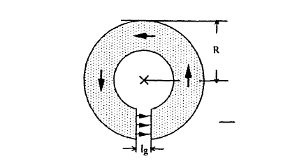
Figure 2.12. Magnetic toroid. The flux and field lines in the toroid are circular. The bold arrows show the direction of the magnetization, and the thin arrows show the direction of the field in the airgap.
magnetostatics. In the absence of external magnetic fields, the magnetostatic energy (1.7) is given by the positive expression \(E_{\text{ms}} = D\mu_{0}M^{2}V/2\). The energy stored outside the magnet, corresponding to half the energy product (section 1.1.1.4), equals \(D(1 - D)\mu_{0}M^{2}V/2\), hence the magnetostatic energy stored inside the magnet is \(D^{2}\mu_{0}M^{2}V/2\). The maximum magnetic field created outside the magnet equals \((1 - D)M\) and is realized at the poles of the ellipsoids. It is of order \(M\) for prolate ellipsoids (needles) and close to zero for very flat oblate ellipsoids (thin films).
Often magnetic particles may be embedded in a matrix, such as epoxy resin or zinc. In this case there exists an effective demagnetizing factor which depends on the volume fraction \(f_{\text{m}}\) of the magnetic particles. If the positions of
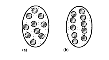
Figure 2.13.Magnetic particles in a matrix: (a) random distribution, (b) chain formation due to magnetostatic interaction
the particles are random (figure 2.13(a)) then
\(D_{\text{eff}} = \frac{1}{3} + f_{\text{m}}(D - \frac{1}{3})\) (2.71)
where \(D\) is the macroscopic demagnetization factor of the sample. This means that \(D_{\text{eff}} = 1/3\) in the dilute limit of \(f_{\text{m}} \approx 0\) and \(D_{\text{eff}} = D\) for \(f_{\text{m}} = 1\). In practice, magnetic particles dispersed in a viscous liquid tend to form columnar structures like that shown in figure 2.13(b). The demagnetizing factor is now given by
\(D_{\text{eff}} = \frac{1}{3}(1 - f_{\text{c}}) + f_{\text{m}}(D - \frac{1}{3})\) (2.72)
where \(f_{\text{c}}\) is the volume fraction of the magnetic particles inside the columns. Putting \(f_{\text{c}} = 1\) and \(f_{\text{m}} = 0\) we obtain the demagnetizing factor \(D_{\text{eff}} = 0\) characteristic of long needles. A typical value encountered in practice is \(f_{\text{c}} = 0.7\).
Microscopic Magnetic Fields
The continuum approach leading to the concept of demagnetizing fields does not take proper account of the atomic structure. Figure 2.14 illustrates the contributions to the local atomic field \(H_{\text{at}} = H + H_{\text{d}}\), where \(H_{\text{d}}(M)\) is the dipolar interaction field acting on the atom. The immediate environment of the site in question has to be dealt with in detail. This is achieved by creating a Lorentz hole which is large compared to the inter-atomic distance. Inside the Lorentz hole, all field contributions must be calculated exactly. Outside the hole, the atomic moments are approximated by a magnetic continuum \(M(r)\). The contribution from inside the Lorentz hole is, in general, anisotropic. In uniaxial magnets, it yields a magnetostatic contribution to \(K_{1}\), which is unrelated to shape anisotropy.
It is important to emphasize that \(H_{\text{at}} \neq H + H_{\text{dm}}\). The difference is seen by considering a central spin in a uniformly magnetized spherical or cubic environment (figure 2.15). Straightforward calculation shows that in both cases \(H_{\text{d}} = 0\) as compared to the normal demagnetizing field \(H_{\text{dm}} = -M/3\). The reason is seen most easily by applying (2.8) to the spherical environment figure 2.15(a).
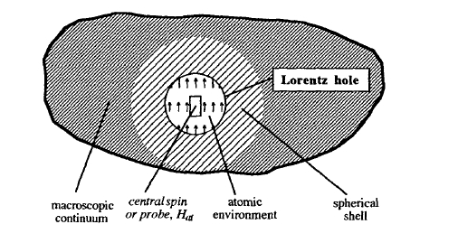
Figure 2.14. The Lorentz-hole construction to calculate the microscopic field \(H_{\text{at}} = H_{\text{d}} + H\).
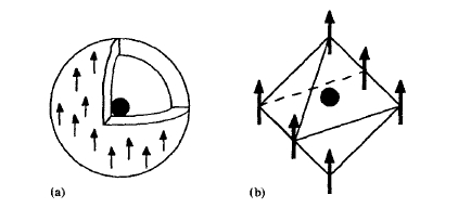
Figure 2.15. Fields acting on central spins in cubic and spherical environments.
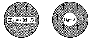
Figure 2.16. Superposition of magnetic fields in magnetic matter (left) and small spherical holes (right). The arrows give the magnetization direction.
In the absence of external fields the only contribution to \(H_{\text{dm}}\) originates from \(\nabla \cdot M\) at the outer surface of the magnet, which gives rise to the demagnetizing field \(-M/3\). By comparison, \(H_{\text{d}}\) contains two opposite surface contributions of equal magnitude: besides the outer surface there is the inner surface surrounding the central spin. Alternatively, dividing the spherical environment into thin shells and using (1.2b) shows that \(H_{\text{d}}\) is proportional to \(\int (3\cos^{2}\theta - 1)\sin\theta \text{d}\theta = 0\). Figure 2.16 summarizes the relation between \(H_{\text{dm}}\) and \(H_{\text{d}}\).
Replacing the sum in (2.64) by an integral yields the interaction energy \(E^{*} = -\mu_{0} \int M \cdot H_{\text{d}} \text{d}V/2\). Comparing this result with (1.5) we see that \(E^{*} = E_{\text{ms}} - \mu_{0}M^{2}V/6\). The difference is the magnetostatic self-energy of the atomic dipoles, which is included in \(E_{\text{ms}}\) but not in \(E^{*}\). However, since the magnetization of permanent magnets is practically field independent, the atomic self-energy amounts to a physically unimportant shift of the zero-point energy.In contrast to the corresponding self-energy contributions, the fields \(H_{\text{d}}\) and \(H_{\text{dm}}\) need to be distinguished properly. Consider, for example, the hypothesis that shape anisotropy is given by the demagnetizing field, so that the shape anisotropy field \(H_{\text{sh}}\) for a sphere would be equal \(-M_{\text{s}}/3\). In fact, the magnetostatic self-energy of a uniformly magnetized sphere is independent of the magnetization direction and \(H_{\text{sh}} = 0\). We see that the shape-anisotropy problem is closely related to the internal-field problem discussed in this subsection, although it cannot be solved without considering incoherent (non-uniform) magnetization states (section 3.2).


