
3. Anisotropy and Coercivity: Exploring Magnetic Behavior
The phenomenon of magnetic hysteresis involves metastable energy minima associated with preferred magnetization directions. Figure 3.1 shows how an external field leads to an irreversible change of the magnetization of a small particle. Two problems arise in the investigation of hysteresis loops of permanent magnets, some of which are shown in figure 3.2. First, one has to trace the origin of the magnetic anisotropy responsible for the energy maxima separating local and global energy minima and, second, extrinsic properties, such as coercivity and energy product, have to be deduced from the energy landscape. The prediction of extrinsic properties is complicated by the fact that truly one-dimensional energy landscapes, such as \(E(\theta)\) in figure 3.1, are rarely encountered in practice. In fact, most magnetization processes of interest are incoherent and the associated energy landscape is multidimensional.
3.1 Magnetic Anisotropy: An Introduction to Its Role in Magnetism
It is often reasonable to assume that the magnitude \(M_{\text{s}}\) of the spontaneous magnetization is a constant independent of orientation and applied field. Magnetic anisotropy means that the energy of a magnetic solid depends on the orientation of the magnetization
\(\mathbf{M} = M_{\text{s}}(\sin\theta\sin\phi\mathbf{e}_{x} + \sin\theta\cos\phi\mathbf{e}_{y} + \cos\theta\mathbf{e}_{z})\) (3.1)
where the unit vector \(\mathbf{e}_{z}\) is parallel to the principal axis. This means that the anisotropy energy becomes a function of the two angles \(\theta\) and \(\phi\). The simple anisotropy expression \(E_{\text{a}}/V = K_{1}\sin^{2}\theta\) (1.23) is widely used, but sometimes it is necessary to take higher-order anisotropy constants into consideration.
The main source of anisotropy in rare-earth permanent magnets is the magnetocrystalline single-ion anisotropy of the rare-earth sublattice. Magnetocrystalline 3d and dipolar anisotropies are of less importance in rare-earth permanent magnets but dominate in transition-metal oxides and 3d metals. Table 3.1 shows that typical 3d and 4f anisotropies of non-cubic magnets are
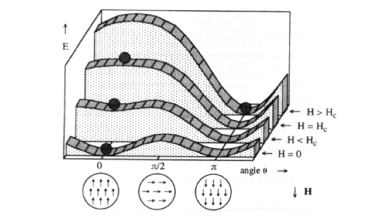
Figure 3.1. Metastable energy minima and coercivity. The permanent spin-up configuration (\(\theta = 0\)) is destabilized by a reverse field until magnetic reversal occurs at the coercivity \(H_{\text{c}}\).
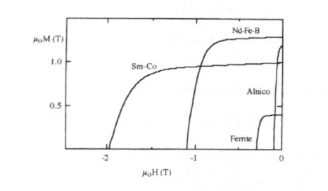
Figure 3.2. Typical second-quadrant demagnetization curves of commercial Nd2Fe14B, SmCo5, Sr ferrite and alnico magnets.
roughly of order 1 MJ m-3 and 10 MJ m-3, respectively. By comparison, magnetostatic dipole interactions give rise to smaller two-ion anisotropies of the order of 0.1–0.5 MJ m-3. This contribution must be distinguished from the magnetostatic shape anisotropy in very small aspherical particles, which is of a similar magnitude.
This section is structured as follows. In subsection 3.1.1 we will give a phenomenological description of magnetic anisotropy; subsection 3.1.2 contains a tentative discussion of anisotropy mechanisms encountered in practice and
Table 3.1. Transition-metal and rare-earth contributions to the room-temperature magnetocrystalline anisotropy. All anisotropies are given in MJ m-3.
| Compound | Symmetry | K1 | K1R | K1T |
|---|---|---|---|---|
| Nd2Fe14B | Tetragonal | 4.9 | 3.8 | 1.1 |
| Sm(Fe11Ti) | Tetragonal | 4.8 | 3.9 | 0.9 |
| Sm2Fe17N3 | Rhombohedral | 8.6 | 9.9 | -1.3 |
| Sm2Co17 | Rhombohedral | 3.3 | 3.7 | -0.4 |
| SmCo5 | Hexagonal | 17.0 | 10.5 | 6.5 |
subsection 3.1.3 is devoted to the magnetocrystalline anisotropy of 3d and 4f sublattices.
Phenomenology of Magnetic Anisotropy: Observations and Insights
Anisotropy Constants
Phenomenologically, the anisotropy energy per unit volume may be expanded in terms of the angles \(\theta\) and \(\phi\). An expression for tetragonal symmetry is
\(\frac{E_{\text{a}}}{V} = K_{1} \sin^{2}\theta + K_{2} \sin^{4}\theta + K_{2}^{(2)} \sin^{4}\theta \cos 4\phi + K_{3} \sin^{6}\theta + K_{3}^{(2)} \sin^{6}\theta \cos 4\phi\) (3.2a)
whereas an expression for hexagonal symmetry1 is
\(\frac{E_{\text{a}}}{V} = K_{1} \sin^{2}\theta + K_{2} \sin^{4}\theta + K_{3} \sin^{6}\theta + K_{3}^{(3)} \sin^{6}\theta \cos 6\phi\). (3.2b)
Here the anisotropy constants \(K_{m}\) and \(K_{m}^{(n)}\) establish a hierarchy of anisotropy contributions of order \(2m\). In section 3.1.2 we will see that the restriction to second-, fourth- and sixth-order terms is motivated by the asphericity of 4f charge clouds. By definition, the anisotropy energy is unchanged by reversing the magnetization, \(E_{\text{a}}(\mathbf{M}) = E_{\text{a}}(-\mathbf{M})\), so there are no odd-order anisotropy contributions2.
The simple expansion (3.2) has a number of limitations: (i) a constant-\(M_{\text{s}}\) one-sublattice approximation is implied; (ii) in a strict sense, the expansion is restricted to cubic, tetragonal and hexagonal crystals; (iii) higher-order
1 Equation (3.2a) can also be used for intermetallics having rhombohedral Th2Zn17 structure, but, in general, rhombohedral magnets may exhibit sin \(3\phi\) and cos \(3\phi\) anisotropy contributions. Equation (3.2b) can be used for cubic crystals, but then only two of the anisotropy constants are independent (section 3.1.1.3).
2 An alternative representation of this symmetry is \(E_{\text{a}}(\theta,\phi) = E_{\text{a}}(\pi + \theta,\pi + \phi)\). We disregard intrinsically unidirectional anisotropy contributions such as that caused by the Dzyaloshinskii–Moriya interaction (section 5.1).
anisotropy contributions are neglected and (iv) the polynomials defined by (3.2) are neither complete nor orthogonal. For example, additional terms such as one in \(\cos^{2}\theta \sin 2\phi\) are needed for intermetallics like R3T29 which have monoclinic symmetry (Wirth et al 1996). The non-orthogonality of the energy terms means, for example, that \(K_{1} \neq 0\) in cubic magnets where there are three equivalent lattice directions (section 3.1.1.3).
A more elegant way to parametrize magnetic anisotropy is to use spherical harmonics, which are both complete and orthonormal (see appendix A5.1). Up to sixth-order contributions, altogether they give rise to 27 anisotropy coefficients \(K_{l}, K_{lm(s)}\), and \(K_{lm(c)}\), where \(0 \leq m \leq l\) and the indices in brackets denote the sine (s) or cosine (c) character of the term. Three of these can be reduced to zero by a suitable choice of axes.
Uniaxial Anisotropy
An approximation which is frequently used is to neglect in-plane anisotropy in crystals with uniaxial symmetry so that (3.2) becomes
\(\frac{E_{\text{a}}}{V} = K_{1} \sin^{2}\theta + K_{2} \sin^{4}\theta + K_{3} \sin^{6}\theta\). (3.3)
In terms of the anisotropy coefficients, (3.3) is
\(\frac{E_{\text{a}}}{V} = \frac{\kappa_{2}}{2}(3\cos^{2}\theta - 1) + \frac{\kappa_{4}}{8}(35\cos^{4}\theta - 30\cos^{2}\theta + 3) + \frac{\kappa_{6}}{16}(231\cos^{6}\theta - 315\cos^{4}\theta + 105\cos^{2}\theta - 5)\). (3.4)
The relation between the uniaxial anisotropy constants and the uniaxial anisotropy coefficients is therefore \(K_{1} = -3\kappa_{2}/2 - 5\kappa_{4} - 21\kappa_{6}/2\), \(K_{2} = 35\kappa_{4}/8 + 189\kappa_{6}/8\) and \(K_{3} = -231\kappa_{6}/16\).
Comparing anisotropy constants and anisotropy coefficients, we see that the order of the anisotropy contributions is denoted differently. Both \(K_{m}\) and \(\kappa_{2m}\) refer to anisotropies of order \(2m\), although the admixture of \(\kappa_{4}\) and \(\kappa_{6}\) to \(K_{1}\) shows that anisotropy constants involve higher-order contributions. This is due to the non-orthogonality of the polynomials in (3.2). By comparison, (3.4) is based on Legendre polynomials (appendix A5.1).
Another shortcoming of the popular expansion (3.3) is the interference of \(\phi\)-dependent terms. In hexagonal and rhombohedral crystals the lowest-order non-uniaxial contribution is the \(K_{3}^{(2)}\) term in (3.2), so that \(K_{1}\) and \(K_{2}\) are well defined uniaxial anisotropy constants. By comparison, \(K_{3}\) is ill defined because it contains a \(\phi\)-dependent admixture of another sixth-order term, namely \(K_{3}^{(2)}\). In this sense, for tetragonal crystals the only well defined uniaxial anisotropy constant is \(K_{1}\).
As we will see in section 3.1.5, the weight of higher-order anisotropy contributions decreases with increasing temperature, so that \(K_{2}\) and \(K_{3}\) are often
Table 3.2. Room-temperature anisotropy constants of some materials.
| Substance | K1 (MJ m-3) | K2 (MJ m-3) |
|---|---|---|
| Fe | 0.048 | 0.015a |
| Ni | -0.005 | 0.005a |
| Co | 0.53 | 0 |
| Fe3O4 | -0.012 | 0.028a |
| Nd2Fe14B | 4.9 | 0.65 |
| Sm2Fe17N3 | 8.6 | 1.46 |
| Sm2Fe17C3 | 7.4 | 0.74 |
| YCo5 | 6.5 | 0.3 |
| Y2Co17 | 0.4 | 0.3 |
| Tm2Co17 | 1.6 | 0.2 |
a \(K_{2}^{(c)}\).
negligible at and above room temperature. Then \(K_{1}\) is the leading anisotropy constant and the preferential magnetization direction is determined by (1.25). For \(K_{1} > 0\) the easy magnetic direction is along the \(c\)- (or \(z\)-) axis, which is called easy-axis anisotropy, whereas \(K_{1} < 0\) leads to easy-plane anisotropy where the easy magnetic direction is anywhere in the \(a - b\) (or \(x - y\)) plane. Since permanent magnets are characterized by strong easy-axis anisotropy, \(K_{1}\) has to be large and positive. Typical orders of magnitude of \(K_{1}\) at room temperature are MJ m-3 in hard magnets and kJ m-3 in soft magnets (tables 3.1 and 3.2). At low temperatures, higher-order anisotropy contributions are more important and may lead to more complicated configurations such as easy cones (section 3.2.3).
Cubic Symmetry
In the case of cubic crystals the leading terms of the expansion of the anisotropy energy per unit volume are
\(\frac{E_{\text{a}}}{V} = K_{1}^{(\text{c})}(\alpha_{1}^{2}\alpha_{2}^{2} + \alpha_{2}^{2}\alpha_{3}^{2} + \alpha_{3}^{2}\alpha_{1}^{2}) + K_{2}^{(\text{c})}\alpha_{1}^{2}\alpha_{2}^{2}\alpha_{3}^{2}\) (3.5)
where \(\alpha_{1} = \cos\theta\), \(\alpha_{2} = \sin\theta\cos\phi\) and \(\alpha_{3} = \sin\theta\sin\phi\) are the direction cosines of the magnetization direction. Analysis of (3.5) shows that \(K_{1}^{(\text{c})} > 0\) favours the alignment of the magnetization along the (001) cube edges, which is called iron-type anisotropy. On the other hand, \(K_{1}^{(\text{c})} < 0\) corresponds to an alignment along the (111) cube diagonals, which is referred to as nickel-type anisotropy. Comparison of (3.2) and (3.5) yields
\(K_{1} = K_{1}^{(\text{c})}\) (3.6a)
\(K_{2} = -\frac{7}{8}K_{1}^{(\text{c})} + \frac{1}{8}K_{2}^{(\text{c})}\) (3.6b)
\(K_{2}^{(2)} = -\frac{1}{8}K_{1}^{(\text{c})} - \frac{1}{8}K_{2}^{(\text{c})}\) (3.6c)
\(K_{3} = -\frac{1}{8}K_{2}^{(\text{c})}\) (3.6d)
\(K_{3}^{(2)} = \frac{1}{8}K_{2}^{(\text{c})}\) (3.6e)
From these equations we see that \(K_{1} = K_{1}^{(\text{c})}\) but \(K_{2} \neq K_{2}^{(\text{c})}\). In terms of section 3.1.1.2, cubic magnets are characterized by \(\kappa_{2} = 0\) but \(K_{1} \neq 0\) due to higher-order anisotropy contributions.
Anisotropy Fields
Fictitious magnetic fields are frequently used in magnetism to reflect the strength of the anisotropy, although the angular dependence of the Zeeman energy \(-\mu_{0}M_{\text{s}}H \cos\theta\) is quite different to that of (3.2). A general anisotropy-field definition is \(\mu_{0}H_{\text{a}} = 2K_{\text{a}}/M_{\text{s}}\), where an effective anisotropy constant \(K_{\text{a}}\) is used rather than the complete set of anisotropy constants. There is, however, no unique way of defining \(K_{\text{a}}\). The simplest definition starts from (3.3) and refers to the maximum energy barrier \(E_{\text{a}}(\pi/2) - E_{\text{a}}(0)\) separating \(\uparrow\) and \(\downarrow\) configurations: \(K_{\text{a}} = K_{1} + K_{2} + K_{3}\). The same expression is obtained by domain-wall analysis (section 3.2.2.2), whereas the initial slopes of the perpendicular magnetization curves (section 3.2.3.2) yield \(K_{\text{a}} = (K_{1} + 2K_{2} + 3K_{3})\). An anisotropy field most closely related to coercivity is obtained from the analysis of nucleation processes in small spherical particles with uniaxial anisotropy (section 3.2.4):
\(H_{0} = \frac{2K_{1}}{\mu_{0}M_{\text{s}}}\). (3.7)
In a strict sense, this equation is valid for \(K_{1} > 0\) only.
Anisotropy-field expressions for cubic magnets do not necessarily agree with the corresponding uniaxial expressions. For instance, the \(K_{1}\) dependence of the ideal nucleation field in cubic crystals is given by \(\mu_{0}H_{0} = 2K_{1}/M_{\text{s}}\) for \(K_{1} > 0\) and \(\mu_{0}H_{0} = -4K_{1}/3M_{\text{s}}\) for \(K_{1} < 0\).
The Physical Origin of Magnetic Anisotropy: Causes and Mechanisms
There are several mechanisms contributing to the anisotropy of permanent magnets. One the one hand, it is necessary to distinguish between the macroscopic shape anisotropy important in small aspherical particles and the magnetocrystalline anisotropy, which is an intrinsic lattice property. The shape anisotropy and a part of the magnetocrystalline anisotropy are two-ion anisotropies caused by magnetostatic dipole interactions. However, the large anisotropy of modern permanent magnets is due to the crystal-field or magneto-electric contribution to the magnetocrystalline anisotropy. The magneto-electric anisotropy mechanism involves electrostatic crystal-field interactions and spin–orbit coupling and is also known as single-ion anisotropy. The latter
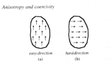
Figure 3.3. Shape anisotropy (schematic). The magnetostatic energy of configuration (b) is higher than that of configuration (a). Shape anisotropy is restricted to small particles, where the inter-atomic exchange ensures a uniform magnetization (section 3.2.4). On the other hand, in non-cubic magnets, the immediate atomic environment (figure 2.14) may give rise to an additional magnetostatic dipole contribution to \(K_{1}\).
mechanism is closely related to the magneto-elastic anisotropy, which may be important in cubic and polycrystalline magnets. In this subsection we will give a short introduction to the main anisotropy mechanisms; detailed discussions of the magneto-electric anisotropies will be given in sections 3.1.3–5.
Magnetostatic Contributions
In non-cubic magnets there is a magnetostatic contribution to the intrinsic, magnetocrystalline anisotropy. Equation (1.3) and figure 2.14 show how this dipolar anisotropy arises from the atomic environment of the magnetic atoms. It is evaluated from lattice sums of the fields due to atomic point dipoles, with the magnetization parallel and perpendicular to the easy axis. In transition-metal rich rare-earth intermetallics, the periodic variation of the local magnetization associated with the layered crystal structure (sections 5.2 and 5.3) yields dipolar contributions to \(E_{\text{a}}\) of the order of \(0.3\) MJ m-3, corresponding to \(\mu_{0}H_{\text{a}} \approx 0.3\) T.
Shape anisotropy is the origin of coercivity in alnico-type magnets and fine-particle powders such as nanocrystalline Fe or CrO2. The idea is illustrated in figure 3.3: the magnetostatic energy of the spin configuration (a) is lower than that of configuration (b), so that the easy magnetization corresponds to the lowest magnetostatic energy. In the case of homogeneously magnetized ellipsoids of revolution, the calculation (section 3.2.3.4) starts from (1.4) and (2.66) and yields the last term in (1.27). Incorporated into the anisotropy expression, that term yields the shape anisotropy constant
\(K_{1,\text{sh}} = \frac{\mu_{0}}{4}(1 - 3D)M_{\text{s}}^{2}\) (3.8)
and the corresponding anisotropy-field expression \(H_{\text{sh}} = (1 - 3D)M_{\text{s}}/2\).
Figure 3.3 indicates that shape anisotropy relies on coherent magnetization states. As we will see in section 3.2.4, particles with diameters larger than about
Table 3.3. Typical atomic radii, shell radii \((r^{2})^{1/2}\), spin-orbit coupling constants and crystal-field energies for 3d and 4f ions (1 Å = 0.1 nm = 100 pm).
| Property | Unit | Transition metals | Rare earths |
|---|---|---|---|
| \(R_{\text{at}}\) | Å | 1.25 | 1.80 |
| \(R_{\text{s}/d}\) | Å | 0.68 | 0.50 |
| \(\lambda\) | K | 500 | 2000 |
| \(E_{\text{CF}}\) | K | 10000 | 100 |
20 nm demagnetize incoherently3, so that (3.8) cannot be used to describe shape anisotropy in bulk magnets or even micrometre-sized particles.
Magneto-electric Anisotropy
The main source of anisotropy in advanced permanent magnets, such as BaFe12O19, SmCo5 and Nd2Fe14B, is the magneto-electric or crystal-field contribution to the magnetocrystalline anisotropy. As opposed to shape and dipolar anisotropy, magneto-electric anisotropy may exceed typical magnetostatic energies by an order of magnitude. This makes it possible to exploit the full saturation magnetization of ferromagnetic materials for permanent magnet applications.
Magneto-electric anisotropy is a combined effect of the crystal-field interaction, spin-orbit coupling and inter-atomic exchange. The orbital motion of the magnetic electrons is subject to the electrostatic crystal field created by all other nuclei and electrons of the crystal. The shape of the electron clouds adapts to the crystal field and reflects the point symmetry of the atomic position. To transform the crystal-field interaction into magnetic anisotropy, the exchange-coupled spins have to communicate with the orbital motion of the electrons, which is realized by spin-orbit coupling. Due to the respective strengths of the spin-orbit coupling, magnetocrystalline anisotropy is more pronounced in 4f compounds than in 3d-based magnets. Typical orders of magnitude of the anisotropy energy per magnetic atom in non-cubic crystals are 1 K and 50 K for 3d and 4f atoms, respectively. However, transition-metal-rich rare-earth intermetallics contain only about 15% rare-earth atoms, so that the transition-metal anisotropy is not necessarily negligible (tables 3.1, 3.2). Table 3.3 shows some of the energy and length scales involved.
The starting point for anisotropy calculations is the Hamiltonian (1.16), which contains ionic, crystal-field and spin-orbit interactions. To illustrate the physics of the anisotropy mechanism we first consider two d orbitals \(|\Psi_{1}\rangle = |xy\rangle\)
3 Note that the onset of incoherent rotation is independent of the single-domain character of a particle (section 3.2).
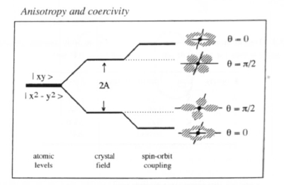
Figure 3.4. Level splitting for the model (3.9). The dashed areas show regions where the 3d charge density is high. The spin-orbit coupling makes the orbitals more running-wave like.
and \(|\Psi_{2}\rangle = |x^{2} - y^{2}\rangle\) in the crystal field shown in figure 2.20. In this case the Hamiltonian simplifies to the \(2 \times 2\) matrix
\(E_{ik} = \begin{pmatrix} A & 0 \\ 0 & -A \end{pmatrix} + 2\lambda \cos\theta \begin{pmatrix} 0 & \text{i} \\ -\text{i} & 0 \end{pmatrix}\) (3.9)
where \(A\) is a parameter giving the electrostatic energy splitting of the two orbitals in the crystal field and \(\theta\) is the angle between the spin direction and the \(z\)-axis. Note that the factor two reflects the magnetic quantum number of the \(d\) orbitals involved. From figures 2.18 and 2.20 we see that the \(|xy\rangle\) orbital is electrostatically less favourable than the \(|x^{2} - y^{2}\rangle\) orbital, so that \(A\) is positive. Equation (3.9) yields the level splitting shown in figure 3.4 and the energy eigenvalues
\(E_{\pm} = \pm\sqrt{A^{2} + 4\lambda^{2} \cos^{2}\theta}\). (3.10)
From figure 3.4 we see that this level splitting gives rise to an easy-axis anisotropy contribution if only one orbital is occupied. By expanding (3.9) in powers of the small quantity \(\lambda^{2}/A^{2}\) we obtain to lowest order the anisotropy energy
\(E_{\text{a}} = \frac{2\lambda^{2}}{A} \sin^{2}\theta\). (3.11)
An equation of this type was first derived by Bloch and Gentile (1931).
It is interesting to discuss (3.9) in the context of the quenching of the orbital moment (section 2.2.2.4). When the magnetization is parallel to the \(z\)-axis the ground-state wavefunction derived from (3.9) is
\(|\psi\rangle = \cos\frac{\chi}{2}|x^{2} - y^{2}\rangle + \text{i}\sin\frac{\chi}{2}|xy\rangle\) (3.12)
Table 3.4. Properties of the magnetic ions following Hund's rules. The energy splitting between the lowest-lying multiplets, \(\Delta E\), is deduced from the spin-orbit coupling constants. All values are given in kelvin.
| Ion | \(\Lambda\) | \(\lambda\) | \(\Delta E\) |
|---|---|---|---|
| 3d1 Sc2+ | 124 | 124 | 310 |
| 3d2 Ti2+ | 88 | 176 | 264 |
| 3d3 V2+ | 82 | 246 | 205 |
| 3d4 Cr2+ | 85 | 340 | 85 |
| 3d5 Fe2+ | -164 | 656 | 656 |
| 3d6 Co2+ | -272 | 816 | 1224 |
| 3d7 Ni2+ | -494 | 987 | 3948 |
| 4f1 Ce3+ | 920 | 920 | 3220 |
| 4f2 Pr3+ | 540 | 1080 | 2700 |
| 4f3 Nd3+ | 430 | 1290 | 2370 |
| 4f4 Pm3+ | 380 | 1540 | 1900 |
| 4f5 Sm3+ | 350 | 1730 | 1230 |
| 4f6 Tb3+ | -410 | 2450 | 2870 |
| 4f7 Dy3+ | -550 | 2730 | 4130 |
| 4f8 Ho3+ | -780 | 3110 | 6240 |
| 4f9 Er3+ | -1170 | 3510 | 8780 |
| 4f10 Tm3+ | -1900 | 3800 | 11400 |
| 4f11 Yb3+ | -4140 | 4140 | 14490 |
where X= arccot\((A/2\lambda)\)is a mixing angle. This means that the admixture of some \(|xy\rangle\) character due to spin-orbit coupling gives rise to an orbital moment
\(\mathbf{m}_{\text{L}} = \frac{4\lambda}{\sqrt{A^{2} + 4\lambda^{2}}} \mu_{\text{B}}\). (3.13)
The orbital moment is therefore only partially quenched and the electron distribution is intermediate figures 2.20(a) and 2.20(b).
The model (3.9) gives a qualitatively correct explanation of 3d anisotropies, although detailed numerical calculations show that it actually overestimates \(K_{1}\). In the case of rare-earth ions the consideration of two degenerate levels is a poor approximation, because the spin-orbit coupling dominates the crystal-field splitting. For example, according to (3.9) the \((x^{2} – y^{2})\) level remains unchanged when the spin is parallel to the \(x\)-axis, but in reality an admixture of other atomic wavefunctions yields unquenched wavefunctions which depend somewhat on the spin direction. Furthermore, one has to consider ionic spin-orbit energies \(\Delta\mathbf{S} \cdot \mathbf{L}\) rather than one-electron contributions \(\lambda\mathbf{s} \cdot \mathbf{l}\). The calculation of the ionic spin-orbit constant \(\Delta\) from the one-electron spin-orbit coupling constant \(\lambda\) is reminiscent of the determination of the ionic moment and yields
\(\Lambda = \lambda/2S\) and \(\Lambda = -\lambda/2S\) for the first and second halves, respectively, of each transition-metal series (Ballhausen 1962). By comparison, typical spin-orbit coupling constants for 3d and 4f ions are of the order of \(10^{4}-10^{5}\) K and 100 K, respectively.
Magneto-elastic Anisotropy
Magnets subject to uniaxial mechanical stress exhibit a magnetostrictive contribution to the magnetic anisotropy. Ultimately, this magneto-elastic anisotropy has a magnetocrystalline origin, since strained crystals can be regarded as unstrained crystals having slightly different atomic positions. Magneto-elastic anisotropy is particularly important in cubic magnets, where uniaxial stress gives rise to uniaxial anisotropy contributions. A good example is hard-magnetic iron (Fe3C4, 5.21), where the carbon causes a martensitic distortion in many cases it is sufficient to consider a uniaxially strained isotropic medium described by the magneto-elastic energy
\(E_{\text{me}} = -\frac{\lambda_{\text{s}}E}{V}(3\cos^{2}\theta – 1)\varepsilon + \frac{E}{2}\varepsilon^{2} – \varepsilon\sigma_{\text{v}}\). (3.14)
Here \(\sigma_{\text{v}}\) denotes the uniaxial stress, \(\varepsilon = \Delta l/l\) is the elongation along the stress axis, \(E\) is Young’s modulus, \(\varepsilon\) is the angle between the magnetization and strain axes. The strength of the magneto-elastic coupling is parametrized by the saturation magnetostriction \(\lambda_{\text{s}}\). To discuss the physical meaning of the dimensionless quantity \(\lambda_{\text{s}}\), we put \(\sigma_{\text{v}} = 0\) and \(\theta = 0\) and minimize the magneto-elastic energy with respect to \(\varepsilon\). The result is that the elongation \(\varepsilon = \lambda_{\text{s}}\), so that we can interpret \(\lambda_{\text{s}}\) as the spontaneous magnetostriction in the magnetization direction. This means that a magnet which is spherical in the paramagnetic state becomes an ellipsoid of revolution in the magnetized ferromagnetic state: for \(\lambda_{\text{s}} > 0\) the ellipsoid is prolate (cigar-like), whereas \(\lambda_{\text{s}} < 0\) leads to an oblate (pancake-like) shape.
In polycrystals, one obtains an average over different crystal orientations. For cubic crystals \(\lambda_{\text{s}}\) is (Kneller 1962)
\(\lambda_{\text{s}} = \frac{3}{2}\lambda_{100} + \frac{3}{2}\lambda_{111}\) (3.15)
where the indices \(\lambda_{100}\) and \(\lambda_{111}\) denote the spontaneous magnetostriction along the cube edges and diagonals, respectively. Experimental room-temperature values of \(\lambda_{\text{s}}\) are \( -7 \times 10^{-6}\) for iron, \( -33 \times 10^{-6}\) for nickel, \(40 \times 10^{-6}\) for Fe3O4, \( -1560 \times 10^{-6}\) for SmFe2, \(1753 \times 10^{-6}\) for TbFe2, \(75 \times 10^{-6}\) for FeCo and practically zero for Fe2Ni80 (Permalloy) (Evett’s 1992, McCurrie 1994). Note that SmFe2 and TbFe2 are cubic Laves-phase compounds, comparatively
large magnitude of their magnetostriction coefficients reflects the pronounced crystal-field interaction of the rare-earth ions.
Since \(\lambda_{\text{s}}\) is very small in most compounds, moderate stress \(\sigma = E\varepsilon\) outweighs the spontaneous magnetostriction and leads to the magneto-elastic anisotropy energy
\(\frac{E_{\text{a}}}{V} = -\frac{\lambda_{\text{s}}\sigma_{\text{v}}}{2}(3\cos^{2}\theta - 1)\). (3.16)
This yields the magneto-elastic contribution
\(K_{1,\text{me}} = \frac{3\lambda_{\text{s}}\sigma}{2}\) (3.17)
to the first anisotropy constant \(K_{1}\). Taking \(\varepsilon = 5\%\), which is typical for tetragonally distorted carbon martensites, \(E = 200\) GPa and \(\lambda_{\text{s}} = 10 \times 10^{-6}\) we obtain the estimate that \(K_{\text{me}} = 0.15\) MJ m-3. This is three times larger than the anisotropy of unstrained bcc iron.
Rare-Earth Anisotropy: Unique Contributions to Magnetic Behavior
The leading anisotropy contribution in rare-earth permanent magnets is the magnetocrystalline anisotropy of the rare-earth sublattice. This is seen most easily by comparing the anisotropies of rare-earth transition-metal intermetallics with those of isostructural intermetallics containing non-magnetic rare earths such as yttrium (table 3.5). As discussed in section 3.1.2.2, magnetocrystalline anisotropy largely originates from the crystal-field interaction and spin-orbit coupling. Since the rare-earth spin-orbit coupling dominates the 4f crystal-field interaction, \(J\) is a good quantum number and lowest-order perturbation theory amounts to the consideration of unquenched ionic wavefunctions \(|\Psi_{\text{J}}\rangle\). In this approximation, the magneto-electric energy is given by \(E_{\text{a}} = \langle\Psi_{\text{J}}|\mathcal{H}|\Psi_{\text{J}}\rangle\).
Expanding the ionic \(N\)-electron wavefunction \(\Psi(\mathbf{r}_{1}, \mathbf{r}_{2}, \ldots, \mathbf{r}_{N})\) in terms of products of \(\phi_{\alpha}(\mathbf{r}_{1})\phi_{\beta}(\mathbf{r}_{2}) \ldots \phi_{\gamma}(\mathbf{r}_{N})\) of atomic 4f orbitals we see that the energy \(E_{\text{a}}\) can be rewritten as
\(E_{\text{a}} = \int V_{\text{cf}}(\mathbf{r})n_{\text{at}}(\mathbf{r}) \text{d}\mathbf{r}\) (3.18)
where \(n_{\text{at}}(\mathbf{r})\) is the ionic charge-density distribution introduced in section 2.2.3. From figures 1.8 and 2.21 we see that the magnetization direction is given by the orientation of charge cloud \(n_{\text{at}}(\mathbf{r})\). Expressing the crystal-field potential \(V_{\text{cf}}\) in terms of the charge density \(\rho(\mathbf{r})\) of the electrons and nuclei that surround the rare-earth atom we obtain
\(V_{\text{cf}}(\mathbf{r}) = -\frac{e}{4\pi\varepsilon_{0}} \int \frac{\rho(\mathbf{R})}{|\mathbf{R} - \mathbf{r}|} \text{d}\mathbf{R}\) (3.19)
and the anisotropy energy
\(E_{\text{a}}(\theta, \phi) = -\frac{e}{4\pi\varepsilon_{0}} \int \frac{n_{\text{at}}(\mathbf{r}; \theta, \phi)\rho(\mathbf{R})}{|\mathbf{R} - \mathbf{r}|} \text{d}\mathbf{r} \text{d}\mathbf{R}\). (3.20)
Table 3.5. Intrinsic properties of some rare-earth intermetallics (Ms and K1 at room temperature). In the case of Y2Co17 and Dy2Co17, the two structures have nearly the same free energy.
| Substance | \(\mu_{0}M_{\text{s}}\) (T) | TC (K) | K1 (MJ m-3) | Structure | |
|---|---|---|---|---|---|
| NdCo5 | 1.23 | 910 | 0.7 | hex. | CaCu5 |
| SmCo5 | 1.07 | 1020 | 17.2 | hex. | CaCu5 |
| YCo5 | 1.06 | 987 | 6.5 | hex. | CaCu5 |
| Pr2Fe14B | 1.55 | 565 | 5.0 | tetr. | Nd2Fe14B |
| Nd2Fe14B | 1.61 | 585 | 4.9 | tetr. | Nd2Fe14B |
| Sm2Fe14B | 1.51 | 621 | -12.0 | tetr. | Nd2Fe14B |
| Y2Fe14B | 1.44 | 566 | 1.1 | tetr. | Nd2Fe14B |
| Dy2Fe14B | 0.72 | 598 | 4.5 | tetr. | Nd2Fe14B |
| Er2Fe14B | 0.95 | 557 | -0.03 | tetr. | Nd2Fe14B |
| Sm(Fe11Ti) | 1.14 | 584 | 4.8 | tetr. | ThMn12 |
| Y(Fe11Ti) | 1.27 | 520 | 1.7 | tetr. | ThMn12 |
| Y(Co11Ti) | 0.93 | 940 | -0.47 | tetr. | ThMn12 |
| Nd2Co17 | 1.39 | 1150 | -1.1 | rhomb. | Th2Zn17 |
| Sm2Co17 | 1.22 | 1190 | 3.3 | rhomb. | Th2Zn17 |
| Dy2Co17 | 0.68 | 1152 | -2.6 | rhomb. | [Th2Zn17, Th2Ni17] |
| Er2Co17 | 0.91 | 1186 | 0.72 | hex. | Th2Ni17 |
| Y2Co17 | 1.25 | 1167 | -0.34 | rhomb. | [Th2Zn17, Th2Ni17] |
| Sm2Fe17 | 1.00 | 389 | -0.8 | rhomb. | Th2Zn17 |
| Y2Fe17 | 0.60 | 327 | -0.4 | hex. | Th2Ni17 |
| Sm2Fe17N3 | 1.54 | 749 | 8.6 | rhomb. | Th2Zn17 |
| Y2Fe17N3 | 1.46 | 694 | -1.1 | hex. | Th2Ni17 |
This equation means that the easy magnetic direction is given by the electrostatic repulsion between the 4f electron cloud and all other charges in the crystal4. Due to the strong ionic-orbital coupling the shapes of the rare-earth electron clouds are well defined spin-orbit (section 2.2.3), although \(n_{\text{at}}\) depends on the angles \(\theta\) and \(\phi\) defined by (3.1), that is on the magnetization direction. On the other hand, the crystal field reflects the atomic positions of the magnetic and non-magnetic rare-earth neighbours. The simple model of figure 1.8 shows a prolate (cigar-like) ion, such as Sm3+, in a uniaxial crystal field.
The transparent dependence of the anisotropy on \(n_{\text{at}}\) and \(\rho\) yields useful qualitative rules. First, in a given crystal-field environment the sign of the rare-earth anisotropy depends on whether the ion is prolate or oblate (section 2.2.3). In particular, Sm and Nd yield opposite anisotropy contributions in isostructural compounds because the Sm3+ and Nd3+ electron clouds are prolate and oblate, respectively.
Here we disregard the limit of very weak intersublattice exchange, where the angular dependence of \(E_{\text{a}}\) is weaker than predicted by (3.20).
respectively. A good example are R2Fe14B compounds (table 3.5): Sm2Fe14B exhibits easy-plane anisotropy as opposed to the easy-axis anisotropy of the permanent magnetic material Nd2Fe14B. Second, (3.20) shows that nonmagnetic atoms contribute to the magnetic anisotropy by modifying the crystal field. A good example here is interstitial nitrogen in Sm2Fe17, which changes the anisotropy from easy-plane to easy-axis.
Point-charge Model and Anisotropy
Equations (3.18) and (3.20) are rather cumbersome integral expressions, and the question arises of whether it is possible to parametrize the crystal field in terms of a few constants. An instructive approach is to assume that the crystal-field charges are located at the sites of the surrounding atoms and act as electrostatic point charges \(\rho(\mathbf{r}) = Q_{i}\delta(\mathbf{r} - \mathbf{R}_{i})\), where \(Q_{i}\) and \(\mathbf{R}_{i}\) are the charge and the position of the crystal-field-creating atom, respectively5. For simplicity, we will restrict ourselves to the cubic (octahedral) and tetragonal environments shown in figure 3.5. Then the crystal-field potential
\(V_{\text{cf}}(\mathbf{r}) = -\frac{e}{4\pi\varepsilon_{0}} \sum_{i = 1}^{N} \frac{Q_{i}}{|\mathbf{R}_{i} - \mathbf{r}|}\) (3.21)
is obtained by putting \(N = 6\) and \(Q_{i} = Q\). Equation (3.18) shows that we need the potential at the ion's site, so that we can expand (3.21) into powers of \(\mathbf{r}\). Neglecting uninteresting isotropic contributions, we obtain to lowest order
\(V_{\text{cf}}(\mathbf{r}) = \frac{35Qe}{8\pi\varepsilon_{0}a^{5}}(x^{2}y^{2} + y^{2}z^{2} + z^{2}x^{2})\) (3.22a)
and
\(V_{\text{cf}}(\mathbf{r}) = \frac{Qe}{4\pi\varepsilon_{0}}\left(\frac{1}{a^{3}} - \frac{1}{c^{3}}\right)(3z^{2} - r^{2})\) (3.22b)
for the cubic and tetragonal environments, respectively. Note the structural similarity between (3.22a) and the \(K_{1}^{(c)}\) term in (3.5). On the other hand, we see that the leading uniaxial crystal-field term (3.22b) vanishes in the cubic limit \(c = a\).
The lowest-order uniaxial contribution (3.22b) can be rewritten as
\(V_{\text{cf}}(\mathbf{r}) = A_{2}^{0}(3z^{2} - r^{2})\) (3.23)
where \(A_{2}^{0}\) is the second-order uniaxial crystal-field parameter. Similarly, (3.22a) can be expressed in terms of fourth-order crystal-field parameters. The crystal-field expansion amounts to a decomposition of the crystal-field potential into
5 This model was introduced by Bethe (1929) to explain optical spectra of solids.
6 The example of pseudocubic intermetallics such as strained PdCo shows that \(a = c\) is not sufficient to ensure cubic anisotropy in complicated compounds.
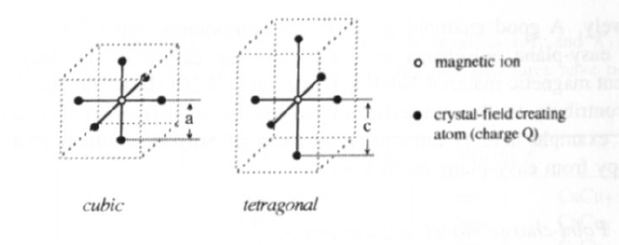
Figure 3.5.1 Cubic and tetragonal point-charge environments characterized by \(a = b = c\) and \(a = b \neq c\), respectively.
orthogonal contributions. Putting (3.23) into (3.18) an examination of the structure of \(n_{\text{at}}\) (section 2.2.3.1) shows that only the second moment \(Q_{2}\) interacts with the \(A_{2}^{0}\) crystal-field contribution. However, in section 2.2.3.1 the angle \(\theta\) refers to the coordinate of the charge, whereas in this chapter \(\theta\) denotes the angle between the magnetization direction and the symmetry axis (c-axis). Incorporating a straightforward rotation of the coordinate frame (section 3.1.3.3) we obtain after a short calculation
\(E_{\text{a}} = \frac{1}{2}Q_{2}A_{2}^{0}(3\cos^{2}\theta - 1)\). (3.24)
Comparing this equation with (1.25) and ignoring a physically unimportant zero-point energy we obtain the lowest-order uniaxial anisotropy constant
\(K_{1} = -\frac{3}{2\Omega_{\text{R}}}Q_{2}A_{2}^{0}\) (3.25)
where \(\Omega_{\text{R}}\) is the crystal volume per rare-earth atom. Higher-order anisotropy contributions are shown in appendix A3.2.
In some sense, (3.25) is the solution of the anisotropy problem: it gives \(K_{1}\) as a function of the shape of the 4f shell, described by \(Q_{2}\), and the crystal environment, described by \(A_{2}^{0}\). In practice, the easy-axis anisotropy required of permanent magnets is achieved by using oblate ions, such as Nd3+, on sites where the crystal-field parameter \(A_{2}^{0}\) is positive and prolate ions, such as Sm3+, in crystalline environments where \(A_{2}^{0}\) is negative. This explains the use of neodymium in R2Fe14B and RT12N intermetallics (section 5.3), whereas samarium is preferred in RCo5, R2Fe17N3 and RT12 intermetallics.
Crystal-field Expansions
A method to deduce crystal-field parameters from expressions such as (3.21) is to exploit the orthogonality and completeness of the spherical harmonics7. In the
Table 3.6. Crystal-field parameters for some intermetallic compounds.
| Compound | \(A_{2}^{0}\) (K \(a_{0}^{-2}\)) | \(A_{4}^{0}\) (K \(a_{0}^{-4}\)) |
|---|---|---|
| R2Fe14B | 300 | -13 |
| R2Fe17 | 34 | -3 |
| R3Fe17N3 | -358 | 39 |
continuous limit one obtains, for example,
\(A_{2}^{0} = -\frac{e}{16\pi\varepsilon_{0}} \int \frac{3R_{z}^{2} - R^{2}}{R^{5}} \rho(\mathbf{R}) \text{d}\mathbf{R}\). (3.26)
For higher-order point-charge contributions see, for example, Hutchings (1964) and appendix A3.3.
One problem is that potentials such as (3.21) obey \(\nabla^{2}V_{\text{cf}} = 0\). In fact, the crystal-field potential is governed by Poisson's equation \(\nabla^{2}V_{\text{cf}} = e\rho/\varepsilon_{0}\), so that delocalized electrons at the rare-earth site give rise to contributions unaccounted for by (3.21). To avoid this difficulty it is convenient to expand \(n_{\text{at}}\) and \(1/|\mathbf{R}-\mathbf{r}|\) rather than \(V_{\text{cf}}\) in spherical harmonics. The result of the calculation for the leading term is
\(A_{2}^{0} = -\int (3\cos^{2}\Theta - 1)\rho(\mathbf{R})W_{2}(R) \text{d}\mathbf{R}\) (3.27)
where \(\cos\Theta = R_{z}/R\),
\(W_{2}(R) = \frac{e}{16\pi\varepsilon_{0}\langle r^{2}\rangle_{4f}}\left(\int_{0}^{R} \frac{\xi^{4}}{R^{3}} f(\xi) \text{d}\xi + \int_{R}^{\infty} \frac{R^{2}}{\xi} f(\xi) \text{d}\xi\right)\) (3.28)
is the second-order crystal-field weight function and \(f(r)\) denotes the radial 4f electron density (section 2.2.3.1). Equation (3.28) describes the radial dependence of the crystal-field interaction, whereas the angular dependence of the crystal field is contained in (3.27). Note that \(W_{2}\) is zero for crystal-field charges at the rare-earth centre (\(R = 0\)) and exhibits a maximum at \(R \approx R_{4f}\). In the limit \(R \gg R_{4f}\), where charge penetration is negligible, \(W_{2}(R) = e/16\pi^{2}\varepsilon_{0}R^{3}\) and (3.26) is reproduced.
Since crystal-field parameters describe the surroundings of the rare-earth ion, they follow the point symmetry of the rare-earth site and should change little in an isostructural series of compounds with different rare earths. Up to minor quenching corrections, the 4f electron clouds exhibit rotational symmetry, so that the description of the rare-earth ions reduces to the three multipole parameters \(Q_{2}\), \(Q_{4}\) and \(Q_{6}\). Note that the angular dependence of the 4f
one-electron wavefunctions causes moments higher than sixth order to vanish. More generally, the maximum index \(m\) of the multipole moments \(Q_{m}\) obeys \(m \leq 2l\), that is \(m \leq 4\) for d ions and \(m \leq 6\) for f ions. Odd multipole moments such as the dipole moment \(Q_{1} = \int n_{\text{at}}(\mathbf{r}) \cos\theta r^{3} \text{d}V\) are zero by symmetry. Note, however, that very strong crystal fields are able to distort the shape of ionic electron clouds, which gives rise to higher-order multipole contributions. Table 3.6 shows the second- and fourth-order uniaxial crystal-field parameters for some rare-earth intermetallics.
Intrinsic Crystal-field Contributions
Equation (3.20) shows that crystal-field interactions obey the superposition principle. This principle is a model concept which is widely used in crystal-field theory and means that the crystal-field contributions of the different rare-earth neighbours can be treated separately so long as their charge density is determined self-consistently. To express the crystal field in terms of the ligands' atomic positions it is convenient to separate the angular dependence from the radial dependence. The lowest-order uniaxial expression is
\(A_{2}^{0} = A_{2}^{\prime}(3\cos^{2}\Theta - 1)\) (3.29)
where the intrinsic crystal-field parameter \(A_{2}^{\prime}\) determines the distance dependence of the atomic crystal-field contributions, whereas the \(\Theta\)-dependent coordination factor gives the angular dependence. For example, azimuthal coordinates as in figure 1.8 correspond to \(\Theta = 0\) and yield \(A_{2}^{0} = A_{2}^{\prime}\), whereas \(\Theta = \pi/2\) describes neighbours in the \(a - b\) or \(x - y\) plane. Note that (3.29) presupposes the charge density of each crystal-field-creating neighbour to be axially symmetric about the line from the rare earth to the neighbour, which is often a fair approximation.
For the point-charge model we obtain from (3.26)
\(A_{2}^{\prime}(R) = -\frac{eQ}{4\pi\varepsilon_{0}} \frac{1}{2R^{3}}\). (3.30)
Measuring \(m\)th-order crystal-field parameters in K \(a_{0}^{-n}\), where \(a_{0}\) is the Bohr radius in Å, and using \(e^{2}/4\pi\varepsilon_{0}k_{\text{B}} = 167102\) K Å, we obtain from (3.30) the numerical estimate \(A_{2}^{\prime} = 23397\) Q/\(eR^{3}\). Due to the multipole character of the crystal-field interactions, higher-order crystal-field parameters exhibit a much stronger dependence on the inter-atomic distance than second-order parameters (Bethe 1929). Numerically, the point-charge model yields \(A_{4}^{\prime} = 1638\) Q/\(eR^{5}\), and \(A_{6}^{\prime} = 229\) Q/\(eR^{7}\). This is one of the reasons for the dominance of the first anisotropy constant \(K_{1}\) in many non-cubic materials. Note that experimental crystal-field charges \(Q\) are typically negative, which indicates that the ligands' electron shells are more important than their nuclei. An exception is hydrogen, which may give rise to zero or positive (protonic) crystal-field charges.
The point-charge model was originally designed to describe non-metallic rare-earth compounds such as garnets Dy3Fe5O12, where the assumption of electrostatic point charges is—to some extent—meaningful. Rare-earth permanent magnets, however, are metals and point charges deduced from the chemical valence of the atoms are screened by the conduction electrons. For example, if nitrogen in Sm2Fe17N3 is assumed to exist as a trinegative ion then its anisotropy contribution is overestimated by a factor of the order of 20. In reality, metallic charges are strongly screened by conduction electrons, which reduces the crystal-field contributions of the neighbours. A metallic extension of the point-charge model is the screened-charge model, where the conduction electrons are described as a weakly disturbed free-electron gas. The second-order intrinsic crystal-field coefficient is given by the asymptotic expression (Skomski 1994)
\(A_{2}^{\prime}(R) = -\frac{eQ}{4\pi\varepsilon_{0}} \frac{e^{-qR}}{2R^{3}}\left(1 + qR + \frac{1}{3}q^{2}R^{2}\right)\) (3.31)
where \(q \approx 2.3 \text{ Å}^{-1}\) is an inverse Thomas-Fermi screening length. In the limit \(q = 0\) this equation reproduces the point-charge result (3.30), so that the screened-charge model can be used to bridge the gap between metallic screening and non-metallic point-charge behaviour, reducing the huge point-charge predictions to a reasonable order of magnitude. However, the description of the intermediate region is only semiquantitative, since rotation of valence-electron orbitals and Friedel oscillations of the electron density contribute to the crystal-field interaction.
From a technical point of view, (3.29) gives an explanation of the angular dependence of the anisotropy energy (3.24). In the coordinate frame of the rare-earth ion, where the z-axis is parallel to the magnetization, the anisotropy energy is the energy necessary to turn the crystal around a rare-earth ion whose magnetization is fixed. By definition, intrinsic crystal-field parameters are angle independent, so that a rotation of the magnetization is equivalent to a rotation of the individual crystal-field charges as described by (3.29).
Equivalent Operators
Equation (3.20) expresses the anisotropy energy in terms of the 4f electron densities of Hund's rules. However, quenching-type deviations from Hund's rules mean that only part of the electrostatic interaction described by (3.20) contributes to the magneto-electric anisotropy. A more general description of the ions is provided by the mean-field Hamiltonian
\(\mathcal{H} = -\frac{\lambda}{\hbar^{2}}\hat{\mathbf{L}} \cdot \hat{\mathbf{S}} - \frac{g\mu_{\text{B}}\mu_{0}}{\hbar} \mathbf{H}_{\text{ex}} \cdot \hat{\mathbf{J}} + \mathcal{H}_{\text{cf}}(\hat{\mathbf{J}})\) (3.32)
where \(\mathcal{H}_{\text{cf}}\) is the crystal-field Hamiltonian expressed in terms of equivalent operators (section 2.2.3.2) and
\(\mathbf{H}_{\text{ex}} = \frac{2(g - 1)}{g\mu_{\text{B}}\mu_{0}\theta}\mathbf{z}_{\text{RT}}\mathcal{J}_{\text{RT}}(\mathbf{s})\) (3.33)
is the exchange field acting on the rare-earth sublattice (section 2.3.2). Interatomic exchange ensures that the local anisotropy contributions translate into a macroscopic anisotropy of the type (3.2). Explicitly,
\(\mathcal{H}_{\text{cf}}(\hat{\mathbf{J}}) = \sum_{n = 0}^{6} \sum_{m = -n}^{n} B_{n}^{m} \hat{O}_{n}^{m}(\hat{\mathbf{J}})\) (3.34)
where \(B_{n}^{m} = \theta_{n}\langle r^{n}\rangle A_{n}^{m}\). Note that the expressions \(B_{n}^{m} \hat{O}_{n}^{m}\) are closely related to the anisotropy coefficients mentioned in section 3.1.1. An advantage of equivalent operators is that they are not restricted to electrostatic crystal-field interactions of type (3.20), but can also include exchange and interatomic hybridization effects. In particular, in rare-earth intermetallics there is an exchange correction of the order of 15% to the dominant second-order electrostatic or Hartree interaction.
The comparatively weak crystal-field interaction of the 4f electrons means that spin-orbit coupling yields unquenched ions obeying Hund's third rule \(J = L \pm S\). As a consequence, intermultiplet excitations characterized by \(J \neq L \pm S\) are negligible in most cases9. However, the relative weakness of the intersublattice exchange, \(\mathcal{J}_{\text{RT}} < \mathcal{J}_{\text{TT}}\), allows intramultiplet excitations (section 2.2.4) which give rise to the temperature dependence of \(\langle J_{z}\rangle\). When \(J_{z} < J\), equations (2.99)–(2.101) show that intramultiplet excitations imply a renormalization of the multipole moments \(Q_{n}\). For instance, the lowest-order uniaxial crystal-field term
\(\mathcal{H}_{\text{cf}}(\hat{\mathbf{J}}) = \theta_{2}A_{2}^{0}\langle r^{2}\rangle_{4f}\hat{O}_{2}^{0}(\hat{\mathbf{J}})\) (3.35)
where \(\hat{O}_{2}^{0}\) is given by (2.87) yields
\(K_{1} = -\frac{3}{2\Omega_{\text{R}}}\theta_{2}A_{2}^{0}\langle r^{2}\rangle_{4f}(3J_{z}^{2} - J(J + 1))\) (3.36)
where \(\langle...\rangle\) denotes the quantum-statistical average with respect to \(J_{z}\). Using (2.99)–(2.101) and including higher-order crystal-field contributions one obtains the uniaxial anisotropy constants
\(K_{1} = -\frac{3}{2\Omega_{\text{R}}}A_{2}^{0}(Q_{2}) - \frac{5}{2\Omega_{\text{R}}}A_{4}^{0}(Q_{4}) - \frac{21}{2\Omega_{\text{R}}}A_{6}^{0}(Q_{6})\) (3.37)
9 A notable exception is Eu3+, where \(\Delta E\) is as small as 300 K. For Sm3+ the splitting is only moderately large (about 1200 K), so that thermal excitations and other perturbations may give rise to moderate intermultiplet excitations (J mixing).
\(K_{2} = \frac{35}{8\Omega_{\text{R}}}A_{4}^{0}(Q_{4}) + \frac{189}{8\Omega_{\text{R}}}A_{6}^{0}(Q_{6})\) (3.38)
\(K_{3} = -\frac{231}{16\Omega_{\text{R}}}A_{6}^{0}(Q_{6})\). (3.39)
To a large extent, the temperature dependence of the magnetocrystalline anisotropy is given by the averages \(\langle Q_{n}\rangle\) (section 3.1.5).
Equation (3.25) is based on the approximation that the intersublattice exchange dominates the crystal-field interaction. In the unrealistic but instructive limit of very weak exchange the order of magnitude of the anisotropy is proportional to \(H_{\text{ex}}\) but independent of \(A_{2}^{0}\).
3d Anisotropy: Insights into Transition Metals and Magnetic Behavior
A common feature of both metallic and non-metallic 3d magnets is the weakness of the spin-orbit coupling compared to inter-atomic interactions. Starting from unperturbed many-electron wavefunctions \(|\Psi_{i}\rangle\), the anisotropy energy is obtained by second-order perturbation theory
\(E_{\text{a}} = E_{0} - \frac{\lambda^{2}}{\hbar^{2}} \sum_{m} \frac{\langle\Psi_{0}|\hat{\mathbf{L}} \cdot \hat{\mathbf{S}}|\Psi_{m}\rangle\langle\Psi_{m}|\hat{\mathbf{L}} \cdot \hat{\mathbf{S}}|\Psi_{0}\rangle}{E_{m} - E_{0}}\). (3.40)
Here the index 0 denotes the ground state, which is assumed to be orbitally non-degenerate. From the point of view of perturbation theory, this equation is equivalent to (3.11). Since the unperturbed wavefunctions \(|\Psi_{i}\rangle\) are independent of the spin direction, we can project out the orbital dependence by performing the summation. This procedure yields the spin Hamiltonian
\(\mathcal{H}_{\text{S}} = -\lambda^{2} \sum_{ik} \Lambda_{ik} \hat{S}_{i} \cdot \hat{S}_{k}\) (3.41)
where
\(\Lambda_{ik} = \frac{1}{\hbar^{4}} \sum_{m} \frac{\langle\Psi_{0}|\hat{L}_{i}|\Psi_{m}\rangle\langle\Psi_{m}|\hat{L}_{k}|\Psi_{0}\rangle}{E_{m} - E_{0}}\). (3.42)
In these equations, the indices \(i\) and \(k\) refer to the \(x\)-, \(y\)- and \(z\)-components of the orbital angular momentum.
The eigenvalues of the \(3 \times 3\) matrix (3.42) yield the lowest-order anisotropy constants. In the uniaxial case, \(\Lambda_{xx} = \Lambda_{yy}\), and the second-order anisotropy energy can be written as \(-D\hat{S}_{z}^{2}\) where \(D = \lambda_{2}(\Lambda_{zz} - \Lambda_{xx})^{10}\).
3d Oxides
To determine the anisotropy of 3d oxides one has to start from ionic wavefunctions \(|\Psi_{i}\rangle\). Figure 3.6 shows the one-electron crystal field splitting for some environments of interest. In reality, the interelectronic interaction leads to a splitting of the one-electron levels as a function of the number of d electrons (Ballhausen 1962).
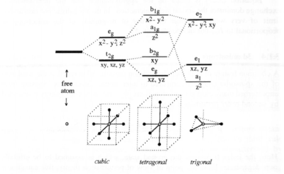
Figure 3.6. Crystal-field splitting energies of one-electron 3d orbitals.
The evaluation of (3.42) yields anisotropy contributions of the type discussed in section 3.1.2.2. A good example is BaFe12O19, where the 12 Fe3+ ions per formula unit occupy three octahedral sites, a tetrahedral site and a trigonal site (figure 5.4). Much of the anisotropy arises from the ferric ions on the trigonal site, which are coordinated by five oxygen atoms and feel a strong uniaxial crystal-field contribution (Fuchikami 1965). Note that trigonal environments are not very effective in quenching the orbital angular momentum, because they are not able to create wavefunctions of the type shown in figure 2.20(a).
Itinerant Anisotropy
In itinerant magnets the inter-atomic hopping is more important than the electrostatic crystal-field interaction, so that the order of magnitude of the level splitting is given by the bandwidth \(W\). In terms of (3.8) and (3.10), the main effect of the inter-atomic hopping is that the unperturbed splitting \(A\) is now \(k\) dependent and \(A \approx W/2\). Table 3.7 summarizes the occurrence of itinerant
Table 3.7. Metallic magnetism. Across a given transition-metal series, \(\lambda\) and \(W\) decrease and increase with increasing atomic number, respectively. Some elements form metallic oxides with narrow bands.
| Element | Degree of electron localization | Spin-orbit coupling | Examples |
|---|---|---|---|
| Late 3d | Local moments in oxides, narrow bands in metals (\(W \sim 5\) eV) | Small (\(\lambda \sim 0.05\) eV) | BaFe12O19, Co |
| 4d | Broad bands in metals, basically paramagnetic* (\(W \sim 10\) eV) | Moderate (\(\lambda \sim 0.5\) eV) | PdFe |
| 5d | Broad bands in metals, basically paramagnetic (\(W \sim 10\) eV) | Rather strong (\(\lambda \sim 1\) eV) | PtCo |
| 4f | Localized in metals and oxides (delocalized for example in CeFe2) | Moderate (\(\lambda \sim 0.2\) eV) | Nd2Fe14B |
| Light 5f | Narrow metallic bands, close to localization (\(W \sim 5\) eV) | Rather strong (\(\lambda \sim 1\) eV) | US |
magnetism. Here emphasis is on 3d metals, but it is worth mentioning that large itinerant anisotropies are observed in 4d, 5d and 5f metals.
Insight into the anisotropy of band electrons is based on the Schrödinger equation
\(E\psi = \frac{\hat{p}^{2}}{2m_{e}}\psi + V(\mathbf{r})\psi + \frac{\hbar}{4m_{e}^{2}c^{2}}(\mathbf{s} \times \nabla V) \cdot \hat{p}\psi\) (3.43)
where \(V(\mathbf{r}) = V(z)\) is a potential periodic in \(z\) modelling a layered compound and the last term is the spin-orbit coupling11. Neglecting interlayer hopping we can use the approximate potential \(V(z) = V_{0}z^{2}/2\), which leads to
\(E_{k} = E_{k0} - \frac{E_{0}}{2}k_{y}^{2}a_{G}^{2} + \frac{E_{0}^{2}}{m_{e}^{2}c^{2}}\sin^{2}\theta\) (3.44)
where \(E_{0}\) is the ground-state energy of the harmonic oscillator described by \(V(z)\) and \(a_{G} \approx 1\) Å is the oscillation amplitude of the electrons in the harmonic potential. This means that electrons subject to a harmonic potential in the \(z\)-direction exhibit easy-plane anisotropy. The total anisotropy energy is obtained by averaging over all \(k\) plane, but its order of magnitude is easily estimated from (3.44). Taking \(k_{y} = 1/a_{G}\) and \(E_{0} = 10\) eV yields the anisotropy energy \(\Delta E/k_{B} = -0.02\) mK, which is much smaller than typical 3d anisotropy energies.
Since Brooks' (1940) attempt to apply the expansions (3.40) to itinerant 3d electrons a large number of band-structure anisotropy calculations have been published. Figure 3.4 shows that each pair of one-electron wavefunctions yields
11 The familiar \(l \cdot s\) form of the spin-orbit coupling is limited to spherical potentials \(V\).
a \(\theta\)-dependent anisotropy contribution if the Fermi level lies between the two levels. Essentially, the magnitude of the anisotropy contributions is given by the energy denominator \(E_{i} - E_{j}\), so that narrow bands yield large anisotropies. On the other hand, the sign of anisotropy depends on the atomic character of the wavefunctions involved. For example, figure 3.4 shows that the spin-orbit coupling between the 'in-plane' \(|xy\rangle\) and \(|x^{2} - y^{2}\rangle\) orbitals yields easy-axis anisotropy. More generally, from the \(l\)-\(s\) matrix elements it follows that the interaction of \(\downarrow\) (or \(\uparrow\)) level pairs yields easy-axis anisotropy for 'in-plane' bands but easy-plane anisotropy for the \(|yz\rangle\), \(|zx\rangle\) and \(|z^{2}\rangle\) orbitals, whose charge distributions have pronounced 'out-of-plane' components. The opposite is true for \(\uparrow\downarrow\) level pairs12, but since the exchange splitting enhances the energy denominator the \(\uparrow\downarrow\) contributions are comparatively small.
In cubic magnets, the choice of a \(z\)-axis has no physical meaning and there is no lowest-order anisotropy contribution. However, the intermetallics of interest as permanent magnets form layered structures and the 3d anisotropy depends on whether the inter-atomic hopping is largest in the \(x\)-\(y\) plane or along the \(z\)-axis. In the former case, the \(|xy\rangle\) and \(|x^{2} - y^{2}\rangle\) bands are very broad and yield a weak easy-axis anisotropy contribution if the \(d\) band is nearly filled. However, this tail contains only a few states, so that for more than about 0.5 \(\downarrow\) holes (Ni, Co) the strong easy-plane contribution of the narrow 'out-of-plane' bands dominates. A further decrease of the number of \(d\) electrons yields another anisotropy zero and both experiment and band-structure calculations show that this frequently falls between Co and Fe. For example, the room-temperature anisotropy \(K_{1}\) for Y2Fe14B and Y2Co14B are \(K_{1} = 1.1\) MJ m-3 and \(K_{1} = -1.2\) MJ m-3, respectively. A notable exception are 2:17 compounds such as Y2(Fe1 - xCox)17, where the transition-metal anisotropy is easy-plane for iron concentrations \(x = 0\) and \(x = 1\) but positive in some intermediate region. These compounds have different local 3d densities on the different sites.
An alternative explanation of the dependence of the anisotropy on the number \(n\) of \(d\) electrons is based on a partial survival of the free-ion multipole moments. Both magnetization measurements and band-structure calculations indicate that the quasi-ionic states of 3d atoms in metals are close to T+ configurations, that is one of the two 4s electrons is accommodated in the 3d band. Indeed, the unquenched quadrupole moment of late 3d elements
\(Q_{2} = \frac{1}{45}(5 - n)(10 - n)(15 - 2n)\langle r^{2}\rangle_{3d}\) (3.45)
exhibits a zero at \(n = 7.5\) \(d\) electrons, that is between the 3d7 (Fe+) and 3d8 (Co+) configurations. The same result is obtained by examining the Stevens coefficient \(\theta_{2}\), which changes sign between 7 and 8 \(d\) electrons. Note that the ultimate reason for the shape of the ionic charge distributions is Hund's second
12 The reason is the transformation behaviour of the Pauli spin matrices: spin-space rotations by an angle \(\pi/2\), that is between parallel and antiparallel spins, correspond to real-space rotations by an angle \(\pi/2\).
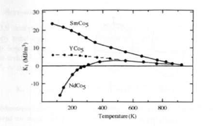
Figure 3.7. The temperature dependence of magnetocrystalline anisotropy in RCo5 compounds.
rule. In band-structure anisotropy calculations, Hund's first and third rules correspond to Stoner exchange and spin-orbit coupling, respectively, but Hund's second rule is ignored because the Stoner exchange is unable to distinguish between the five d subbands. To include Hund's second rule in band-structure calculations one has to add an \(L_{z}^{2}\) or orbital polarization term to the Stoner-type exchange (section 2.4.2.2).
Temperature Dependence of Magnetic Anisotropy: Key Trends and Effects
The temperature dependence of the magneto-electric anisotropy is of great importance in permanent magnetism: aside from secondary magnetic viscosity effects (section 3.4) it determines the temperature dependence of the coercivity. Figure 3.7 shows the temperature dependence of the anisotropy of some RCo5 intermetallics. At low temperatures, there is a large difference between that for SmCo5 and NdCo5. This is due to the different shapes of the rare-earth electron clouds, as discussed in section 2.2.3 and 3.1.3. With increasing temperature the rare-earth contribution becomes smaller and the anisotropy approaches the value of YCo5, where yttrium acts as a non-magnetic rare earth. This behaviour is not restricted to RT5 intermetallics: rare-earth anisotropy contributions dominate at low temperatures, whereas the small anisotropy in the vicinity of the critical point is determined by the transition-metal sublattice.
Equations (2.98)–(2.101) and (3.37)–(3.39) show the intramultiplet origin of the temperature dependence of the rare-earth anisotropy. The exchange interaction favours complete spin alignment, \(J_{z} = J\), but thermal excitations lead to the admixture of states characterized by \(J_{z} < J\). Figure 3.8 shows the real-space meaning of these excitations. At low temperatures the exchange field assures an aspherical charge distribution, but at moderate temperatures—that is above the rare-earth transition-metal intersublattice coupling temperature \(T_{\text{RT}}\)—thermal excitations produce a smearing of the 4f charge cloud.
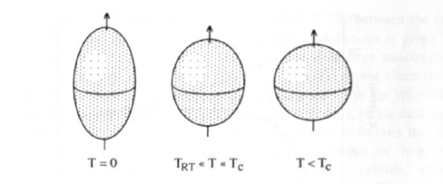
Figure 3.8. Thermal smearing of an aspherical 4f charge cloud, responsible for the temperature variation of the rare-earth contribution to \(K_{1}\). In this figure we have ignored the asphericity of the 4f electron cloud induced by an external magnetic field which gives rise to an anisotropic susceptibility above \(T_{C}\).
Anisotropy and Magnetization of One-Sublattice Magnets
Let us start with the classical Heisenberg model, where the \(J_{z}\) dependence of the multipole moments (2.99)–(2.101) reduces to Legendre polynomials \(P_{n}(\cos\theta)\). As a consequence, \(K_{mn}(T)/K_{m0}(T) = (P_{2m}(\cos\theta))\). For example, the temperature dependence of the lowest-order uniaxial anisotropy contribution is given by \(\langle P_{2}\rangle = \langle(3\cos^{2}\theta - 1)/2\rangle\). To calculate the thermal averages involved we have to evaluate integrals of the type
\(I_{m}(E_{\text{ex}}/k_{\text{B}}T) = \int_{0}^{\pi} \exp\left(\frac{E_{\text{ex}}}{k_{\text{B}}T} \cos\theta\right) \cos^{m}\theta \sin\theta \text{d}\theta\) (3.46)
where \(E_{\text{ex}}\) is an exchange-energy parameter. In the low-temperature limit, \(I_{m}(x) = (1 - mx)\exp(x)/x\) so that \(\langle\cos^{m}\theta\rangle = 1 - mk_{\text{B}}T/E_{\text{ex}}\), \(M_{s}/M_{0} = 1 - k_{\text{B}}T/E_{\text{ex}}\) and \(\langle P_{m}\rangle = 1 - m(m + 1)k_{\text{B}}T/2E_{\text{ex}}\). These relations yield the famous \(m(m + 1)/2\) power law13
\(\frac{K_{m/2}(T)}{K_{m/2}(0)} = \left(\frac{M_{s}}{M_{0}}\right)^{m(m + 1)/2}\). (3.47)
In other words, second-, fourth- and sixth-order anisotropy contributions are proportional to the third, 10th and 21st powers of the magnetization, respectively. A qualitative conclusion which can be drawn from the \(m(m + 1)/2\) power law is that the temperature dependence of higher-order anisotropy contributions is very pronounced.
To derive (3.47) we have used a low-temperature approach, but in practice the validity of that equation is not necessarily restricted to very low temperatures. For example, in one-sublattice magnets such as bcc iron it is obeyed up to about 0.65 \(T_{C}\) (see section 3.1.5.3). The reason is that (3.47) reflects the symmetry of the anisotropy terms rather than a particular finite-temperature model.
Rare-earth Anisotropy
Figure 3.9 analyses the temperature dependence of \(K_{1}\) in terms of the leading anisotropy mechanisms. The low-temperature plateau is a quantum effect: the non-zero level spacing \(\Delta E\) associated with the eigenvalues \(-J \leq J_{z} \leq J\) of the mean-field Heisenberg model (figure 2.29(a)) suppresses thermal excitations below \(T_{0} \approx \Delta E/k_{\text{B}}\).
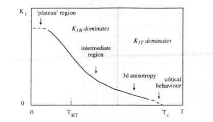
Figure 3.9. The temperature dependence of magnetocrystalline anisotropy if both \(K_{1T}\) and \(K_{1R}\) are positive (schematic). \(K_{2R}\) and \(K_{3R}\) may be important far below \(T_{RT}\).
In the practically important intermediate region above \(T_{RT}\) but well below \(T_{C}\) one has to consider quasi-paramagnetic rare-earth ions in an exchange field of the transition-metal sublattice. This region is characterized by the increasing sphericity of the 4f charge clouds (figure 3.8). Using the high-temperature limit of (3.46) we obtain the power-law expression
\(\frac{K_{1R}(T)}{K_{1R}(0)} = \frac{E_{\text{ex}}^{2}}{15k_{\text{B}}^{2}T^{2}}\). (3.48)
\(E_{\text{ex}}\) is proportional to the magnetization of the transition-metal sublattice, but well below \(T_{C}\) we can replace it by a constant value of order \(k_{\text{B}}T_{RT}\). Due to the classical character of (3.46) the validity of (3.48) is restricted to \(T \gg T_{0}\).
Transition-metal Sublattice Anisotropy
At high temperatures the contribution (3.48) is negligible and the remaining anisotropy arises from the transition-metal sublattice as indicated in figure 3.9. Neglecting the band-structure instability of the magnetic moment (section 2.4.3.3) we can use (3.46) to calculate the quasi-classical mean-field averages \(\langle\cos\theta\rangle\) and \(\langle P_{2}(\cos\theta)\rangle\). As in (2.95), the magnetization is given by
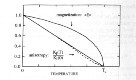
Figure 3.10. Finite-temperature behaviour of the classical mean-field Heisenberg model. The dashed curve is the \(n(n + 1)/2\) power-law anisotropy prediction.
the Langevin expression
\(\langle\cos\theta\rangle = \coth\frac{E_{\text{ex}}}{k_{\text{B}}T} - \frac{k_{\text{B}}T}{E_{\text{ex}}}\) (3.49)
whereas the average \(P_{2}(\cos\theta)\) yields
\(\frac{K_{1}(T)}{K_{1}(0)} = \frac{3k_{\text{B}}^{2}T^{2}}{E_{\text{ex}}^{2}} + 1 - \frac{3k_{\text{B}}T}{E_{\text{ex}}} \coth\frac{E_{\text{ex}}}{k_{\text{B}}T}\). (3.50)
Putting \(\coth(E_{\text{ex}}/k_{\text{B}}T) = \langle\cos\theta\rangle + k_{\text{B}}T/E_{\text{ex}}\) into (3.50) and using the relations \(E_{\text{ex}} = z\mathcal{J}_{0}\langle\cos\theta\rangle\) and \(k_{\text{B}}T_{\text{C}} = z\mathcal{J}_{0}/3\) (section 2.3.2) we obtain the surprisingly simple result
\(K_{1}(T) = K_{1}(0)\left(1 - \frac{T}{T_{\text{C}}}\right)\). (3.51)
By comparison, (3.49) is an implicit equation for the magnetization (figure 3.10).


