
Magnetic Properties of Intermetallic Compounds: Their Relevance to Permanent Magnetss
In the search for new technological magnetic materials, the most interesting for use as permanent - magnet materials would be those exhibiting large values of saturation magnetization and magnetic anisotropy. As noted in the previous chapter, some of the hexagonal \(\text{Co}_{5}\text{R}\) intermetallic compounds exhibit this combination of properties. In fact, they exhibit the largest magnetocrystalline anisotropy energies with substantial values of saturation magnetization at room temperature that are known. Permanent magnets based on these materials have now been made with previously unattainable coercivities and energy products.
The Co₅R Phases: Structure, Magnetic Behavior, and Applications
The early work [1 - 3] on these materials established that the magnetization of the light - R sublattice (atomic number less than that of Gd) coupled ferromagnetically to the magnetization of the Co sublattice, while the opposite is true for the heavy - R elements, rendering these latter materials ferrimagnetic with compensation points (temperatures where the magnetizations of the magnetic sublattices cancel). Figure 3.1
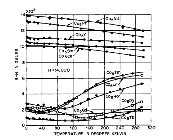
Figure 3.1 Variation of magnetization (\(B - H\)) with temperature for \(\text{Co}_{5}\text{R}\) compounds (after Nesbitt et al. [1, 2]).
shows the magnetization curves for these materials.* The minima exhibited by the heavy \(\text{Co}_{5}\text{R}\) phases, as well as the results of other experiments [3], indicate the existence of compensation points. A unique temperature where \(B - H = 0\) was not observed, possibly due to local inhomogeneities in the polycrystalline samples or to a complex magnetic structure that does not change with temperature in a simple manner. In order to circumvent the high anisotropy, loose powders of these materials were aligned in the field. This procedure yielded values of magnetization (Figure 3.1) that essentially correspond to saturation, even though the measurement field was only 14,000 Oe. High Curie points are exhibited (Table 3.1) by some of these materials [4 - 8], the highest value being \(724^{\circ}\text{C}\) for \(\text{Co}_{5}\text{Sm}\). It is apparent from Figure 3.1 that the light \(\text{Co}_{5}\text{R}\) materials exhibit higher saturation magnetizations and are thus technologically more useful.
As pointed out in Chapter II, the magnetic behavior of the rare - earth atoms is due to the unpaired inner 4f electrons. Thus, the atomic moments are localized, and it has been established that interatomic exchange occurs indirectly via polarization of the conduction electrons. The exchange interaction is an oscillating function of distance, decaying at large distances (Ruderman - Kittel - Kasuya - Yosida theory) [9]. For the rare - earth atoms of atomic number greater than that of Gd, the total angular momentum \(|J|=|L| + |S|\), and for atomic numbers less than that of Gd, \(|J|=|L|-|S|\). (For Gd, \(|J| = |S|\).) In the \(\text{Co}_{5}\text{R}\) phases, the spins on the R atoms are coupled
* The isostructural \(\text{Ni}_{5}\text{R}\) compounds are paramagnetic at room temperature because, on a rigid band model, the three valence electrons of each R atom fill the 3d band of the Ni. Pure Ni effectively has 0.6 hole in the d band per atom; thus the \(\text{Ni}_{5}\) d band has three holes to accommodate the three valence electrons per rare - earth ion.
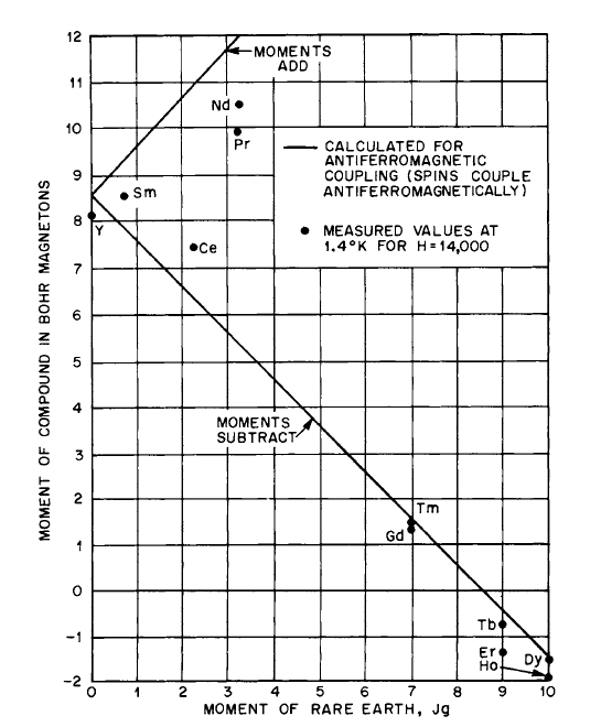
Figure 3.2 Variation of magnetic moments of \(\text{Co}_{5}\text{R}\) compounds with moment of the rare - earth element (after Nesbitt et al. [1, 2]).
antiparallel to the spins on the Co atoms. For the light rare - earth atoms, the 4f spin and orbital moments are opposed to one another and the net magnetic moment \(Jg\) is coupled ferromagnetically to the Co. For Gd and the heavier rare - earth atoms, \(S\) and \(L\) are parallel to one another, so \(Jg\) is antiparallel to the Co moment, leading to two - sublattice ferrimagnetism, and thus to a lowering of the total magnetization and resulting in the appearance of compensation points.
The magnetic behavior of the \(\text{Co}_{5}\text{R}\) compounds can be interpreted in terms of a two - sublattice model, which can be deduced by examining Figure 3.2. \(\text{Co}_{5}\text{Y}\) exhibits a moment of \(8.3\ \mu_{B}\), approximately equal to the value computed on the basis of the moment of metallic cobalt. The heavy rare earths couple antiferromagnetically, and the moments of these compounds can be calculated by simply subtracting from the moment of five metallic cobalt atoms the \(Jg\) value of the rare - earth ion. This procedure yields the solid line shown in the figure. The experimental values are in good agreement with the calculated values. For the light rare - earth elements, the measured moments suggest ferromagnetic coupling between the Co and rare - earth atoms.
The \(L\) and \(S\) (and \(J\)) coupling scheme discussed above suggests still another experiment to support ferro - and ferrimagnetic behavior of these phases. Since, in these 5:1 compounds, the moments of the light rare - earth elements add to that of the cobalt and the moments of the heavy rare - earth elements subtract, it should be possible to devise a composition in which these moments cancel each other. This has been done as shown in Figure 3.3. The rare - earth moments cancel in the compound \(\text{Co}_{5}\text{Gd}_{0.3}\text{Nd}_{0.7}\), where the ratio of Nd to Gd is that required to reduce the total moment to that of \(\text{Co}_{5}\text{Y}\). As discussed in Reference 11, Chapter IV, the magnetization behavior of these compounds and their alloys can be utilized to control
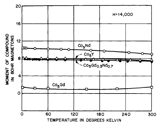
Figure 3.3 Variation of magnetic moment with temperature for \(\text{Co}_{5}\text{Y}\), \(\text{Co}_{5}\text{Nd}\), \(\text{Co}_{5}\text{Gd}\), and \(\text{Co}_{5}\text{Gd}_{0.3}\text{Nd}_{0.7}\). These results show that the moments of Nd and Gd are antiparallel and the ratio of Nd to Gd in \(\text{Co}_{5}\text{Gd}_{0.3}\text{Nd}_{0.7}\) is that required to reduce the total moment to that of \(\text{Co}_{5}\text{Y}\).
the temperature coefficients of permanent magnets based on these materials.
The use of the moment of Co based on cobalt metal for the above discussion is reasonable. Nevertheless, in a given lanthanide - cobalt binary system, the cobalt moment may vary with composition [1 - 3, 10 - 14]. As an example, consider the Gd - Co system (Figure 3.4) [12]. The antiparallel coupling of Gd (\(S\) only) to the cobalt moment results in a lower moment. Since the moment of Gd is well localized, the effective moment of Co can be computed by assuming the Gd moment to remain constant. The drop in moment of Co as the Gd con -
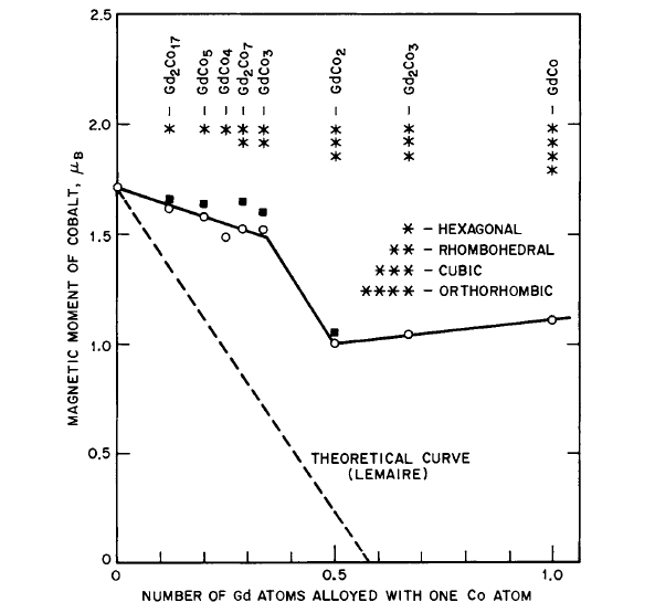
Figure 3.4 Variation of the cobalt moment in Gd - Co intermetallic compounds: ○—experimental points; ■—results according to Lemaire [13] (after Strydom and Alberts [12]).
tent increases was explained on a rigid band basis by Lemaire [13] in that the 3d band of cobalt is gradually filled by the three valence electrons of Gd. As can be seen, the observed moments are, however, much larger than the theoretical (dashed curve). Even the postulated partial filling of split
cobalt d sub - bands [15, 16] by the s - d valence electrons of Gd cannot explain the subsequent increase in Co moment with increasing Gd content. An alternative explanation [12] of the subsequent rise in Co moments makes use of the fact that the exchange interaction is indirect via polarization of the conduction electrons, and as more Gd is added, the polarized electrons begin to contribute substantially to the moment.
Magnetic structures of \(\text{Co}_{5}\text{Y}\), \(\text{Co}_{5}\text{Ho}\), and \(\text{Co}_{5}\text{Nd}\) were determined by neutron diffraction studies [17 - 19]. For \(\text{Co}_{5}\text{Y}\), the Co moments are coupled ferromagnetically along the \(c\) axis. The Co moment required to give agreement between observed and calculated intensities was nearly the same as that exhibited by metallic cobalt [17]. For \(\text{Co}_{5}\text{Ho}\) at room temperature, the Co and Ho moments are opposed; the Ho moments are directed along an axis located \(22^{\circ}\) from the \(c\) axis. For \(\text{Co}_{5}\text{Nd}\), the easy axis of magnetization is the \(c\) axis at 300 K and above, but rotates into the basal plane as the temperature is decreased, so that at \(\sim230^{\circ}\text{K}\) the easy axis of magnetization is in the basal plane [18].
The \(\text{Co}_{5}\text{R}\) compounds exhibit a large magnetocrystalline anisotropy, and the "wormlike" domain structure of \(\text{Co}_{5}\text{Sm}\), typical of uniaxial permanent - magnet materials, was demonstrated by the Kerr magneto - optic effect [3] (see Figure 1.4, Chapter I). Qualitative confirmation of the possible existence of large magnetocrystalline anisotropy was demonstrated by Hubbard et al. [20] when they measured an intrinsic coercivity of 8000 Oe on \(- 100+200\) mesh \(\text{Co}_{5}\text{Gd}\) powder. As pointed out in Chapter I, if magnetocrystalline anisotropy is the dominant anisotropy, the maximum theoretical coercivity (or anisotropy field \(H_{A}\)) is equal to \(2K/M_{s}\). Thus, a large coercivity suggests the possibility of a large magnetocrystalline anisotropy. Strnat and his associates [4 - 8] subsequently determined \(K_{u}\) and \(H_{A}\) from magnetization data obtained in the easy and hard directions (as described in Chapter I, Figure 1.14). They obtained values in excess of \(10^{7}\text{ ergs/cm}^{3}\) and 100 kOe respectively for \(\text{Co}_{5}\text{Y}\) and other \(\text{Co}_{5}\text{R}\) phases (Table 3.1). These results, taken in conjunction with the high saturation exhibited by the light \(\text{Co}_{5}\text{R}\) compounds, stimulated activity to prepare permanent magnets based on powders (see Chapter V). Theoretical maximum energy products \([(BH)_{\text{max}} = 4\pi M_{s}^{2}]\) could be in excess of \(35\times10^{6}\text{ G - Oe}\) (Table 3.1). Recently [21] anisotropy values for some solid solutions of \(\text{Co}_{5}\text{R}\) and \(\text{Cu}_{5}\text{R}\) have been obtained. For the alloy \(\text{Co}_{3.5}\text{CuFe}_{0.5}\text{Ce}_{1.09}\), the values of \(K_{u}\) were 4.5, 4.5, 3.5, and \(2.1\times10^{7}\text{ erg/cm}^{3}\) for the respective temperatures of 4.2, 68, 150, and \(300^{\circ}\text{K}\); for the alloy \(\text{Co}_{3.5}\text{CuFe}_{0.5}(90\%\ \text{Ce}\ \text{misch metal})_{1.0}\), the values of \(K_{u}\) were
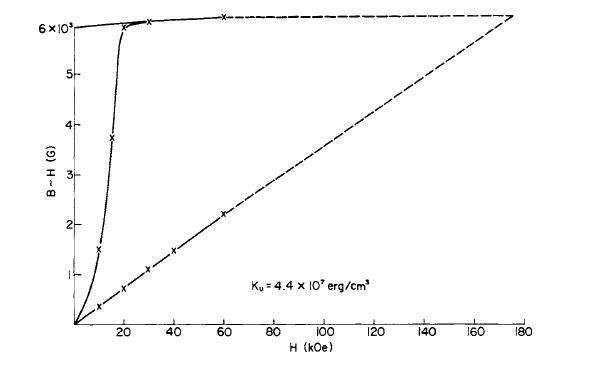
Figure 3.5 Magnetization at \(4.2^{\circ}\text{K}\) in the easy and hard directions as a function of applied field for \(\text{Co}_{3.5}\text{CuFe}_{0.5}\text{Ce}_{1.09}\). Here \(K_{u}\) computed from the extrapolated anisotropy field is \(\sim4.5\times10^{7}\text{ ergs/cm}^{3}\).
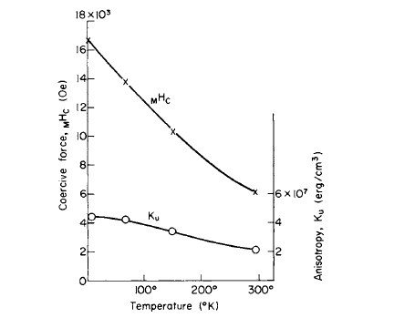
Figure 3.6 Figure Variation of \(K_{u}\) and \(_{M}H_{c}\) with temperature for \(\text{Co}_{3.5}\text{CuFe}_{0.5}\text{Ce}_{1.09}\).
3.8, 3.8, 3.6, and \(2.9\times10^{7}\text{ erg/cm}^{3}\) for the respective temperatures of 4.2, 68, 150, and \(300^{\circ}\text{K}\). \(K_{u}\) is computed from the formula \(H_{A}=2K_{u}/M_{s}\). Measurements were made in fields up to 60 kOe. Typical magnetization curves at \(4.2^{\circ}\text{K}\) for the easy and hard directions are shown in Figure 3.5. The variation of \(K_{u}\) and \(_{M}H_{c}\) with temperature is shown in Figure 3.6. In this instance, when the temperature is lowered, \(_{M}H_{c}\) increases at a greater rate than \(K_{u}\).
Magnetocrystalline Anisotropy: The Key to Magnetic Alignment and Performancey
The magnetic anisotropy energy \(E_{a}\) of the \(\text{Co}_{5}\text{R}\) phases may be written\(E_{a}=K_{1}\sin^{2}\theta + K_{2}\sin^{4}\theta+\cdots\) where \(\theta\) is the angle the magnetization makes with the \(c\) - axis of the crystal, and \(K_{1}\) and \(K_{2}\) are anisotropy constants. In some cases, the first term is sufficient for computing the anisotropy energy.
Recently [22], \(K_{1}\) and \(K_{2}\) for \(\text{Co}_{5}\text{Y}\), \(\text{Co}_{5}\text{Ce}\), \(\text{Co}_{5}\text{Pr}\), \(\text{Co}_{5}\text{Nd}\), and \(\text{Co}_{5}\text{Sm}\) were determined from measurements on single -
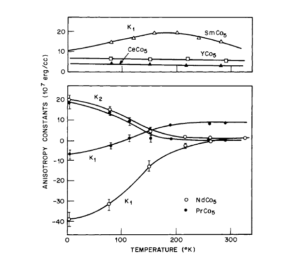
Figure 3.7 Variation of the anisotropy constants \(K_{1}\) and \(K_{2}\) with temperature for \(\text{Co}_{5}\text{Y}\), \(\text{Co}_{5}\text{Ce}\), \(\text{Co}_{5}\text{Pr}\), \(\text{Co}_{5}\text{Nd}\), and \(\text{Co}_{5}\text{Sm}\) (after Tatsumoto et al. [22]).
crystal spheres. For \(\text{Co}_{5}\text{Y}\), \(\text{Co}_{5}\text{Ce}\), \(\text{Co}_{5}\text{Pr}\), \(\text{Co}_{5}\text{Nd}\), and \(\text{Co}_{5}\text{Sm}\), \(K_{1}(0^{\circ}\text{K}) = 6.5, 5.5, - 7, - 40\), and \(10.5\times10^{7}\text{ erg/cm}^{3}\) respectively and \(K_{2}(0^{\circ}\text{K})=\sim0, \sim0, 18, 19\), and \(0\times10^{7}\text{ erg/cm}^{3}\) respectively. The variation of \(K_{1}\) and \(K_{2}\) with temperature is shown in Figure 3.7. For the Y, Ce, and Sm compounds, \(K_{1}\) is positive at all temperatures and \(K_{2}\) is negligible. The broad maximum for \(\text{Co}_{5}\text{Sm}\) is suggested [22] as being due to the admixture of higher - lying Sm J states with the ground state. For the Nd and Pr compounds, \(K_{1}\) changes sign with decreasing temperature and \(K_{2}\), positive in value, becomes larger. The variation of \(K_{1}(0^{\circ}\text{K})\) and \(K_{2}(0^{\circ}\text{K})\) in the \(\text{Co}_{5}\text{Y}_{1 - x}\text{Nd}_{x}\) system is shown in Figure 3.8.
The manner in which the easy direction of magnetization for \(\text{Co}_{5}\text{Pr}\) and compositions in the \(\text{Co}_{5}\text{Y}_{1 - x}\text{Nd}_{x}\) system varies with temperature is shown in Figure 3.9. The data were obtained by torque measurements and are consistent with the behavior of \(K_{1}\) and \(K_{2}\) with temperature. Note that the critical temperatures at which the easy axis of magnetization begins
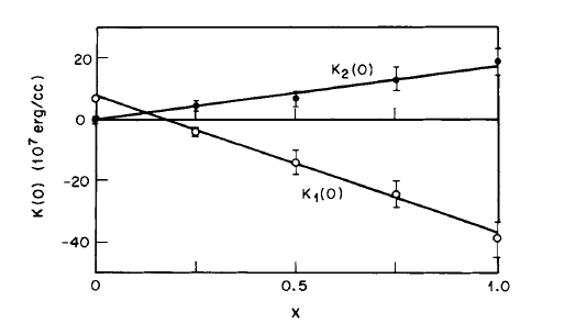
Figure 3.8 Variation of \(K_{1}(0^{\circ}\text{K})\) and \(K_{2}(0^{\circ}\text{K})\) with composition in the \(\text{Co}_{5}\text{Y}_{1 - x}\text{Nd}_{x}\) system (after Tatsumoto et al. [22]).
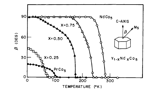
Figure 3.9 Variation of the easy direction of magnetization with temperature in the \(\text{Co}_{5}\text{Y}_{1 - x}\text{Nd}_{x}\) system and for \(\text{PrCo}_{5}\) (after Tatsumoto et al. [22]).
to rotate away from the \(c\) axis is \(\sim105^{\circ}\text{K}\) for \(\text{Co}_{5}\text{Pr}\) and \(283^{\circ}\text{K}\) for \(\text{Co}_{5}\text{Nd}\), in agreement with the neutron diffraction results [18].
The Co₁₇R₂ and Fe₁₇R₂ Phases: Exploring Their Magnetic and Structural Characteristics
As noted in Chapter II, the structures of these phases are closely related to the \(\text{CaCu}_{5}\) type; they are of interest in permanent - magnet studies because some exhibit large saturation magnetization and high Curie points. Most of the saturation magnetizations of the \(\text{Co}_{17}\text{R}_{2}\) compounds are larger than those exhibited by the \(\text{Co}_{5}\text{R}\) phases because of the greater concentration of 3d atoms. Their magnetic behavior can also be interpreted in terms of a two - sublattice model in which the spin angular momentum of the R atoms is antiparallel to the
magnetic moment of the Co and Fe [23, 24]. At room temperature, \(\text{Co}_{17}\text{Y}_{2}\) does not show a unique easy axis; it exhibits an easy plane with no anisotropy within the plane and consequently cannot be used for crystal anisotropy - controlled permanent magnets [25]. The \(c\) axis is the hard axis of magnetization. \(\text{Co}_{17}\text{Ce}_{2}\), \(\text{Co}_{17}\text{Pr}_{2}\), and \(\text{Co}_{17}\text{Nd}_{2}\) also appear to exhibit an easy basal plane, while \(\text{Co}_{17}\text{Sm}_{2}\), \(\text{Co}_{17}\text{Er}_{2}\), and \(\text{Co}_{17}\text{Tm}_{2}\) exhibit an easy axis [26 - 28]. However, some ternary alloys in several \((\text{Co}_{1 - x}\text{Fe}_{x})_{17}\text{R}_{2}\) systems, where \(R = Y\), Ce, and Pr, exhibit
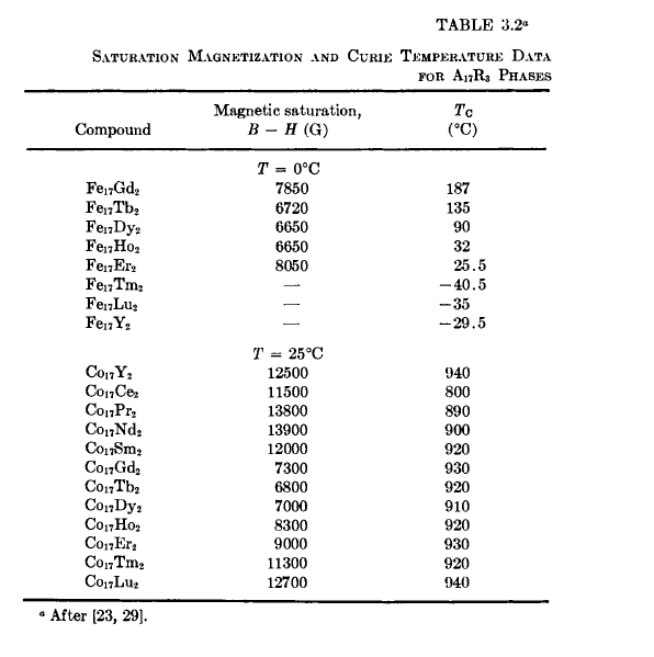
an easy axis parallel to the crystallographic \(c\) axis [30, 31]. Table 3.2 contains saturation and Curie point values for many of the \(\text{Fe}_{17}\text{R}_{2}\) and \(\text{Co}_{17}\text{R}_{2}\) compounds. It is apparent from this table that the \(\text{Co}_{17}\text{R}_{2}\) compounds have superior properties in regard to saturation and Curie point values compared to those of \(\text{Fe}_{17}\text{R}_{2}\).


