

6.2 Static Applications of Magnetism: Principles and Uses
Uniform Magnetic Fields: Generation, Properties, and Applications
It is not obvious that permanent magnets can be used to generate uniform fields, because the magnetic field produced by a point dipole of moment \(m\ A\ m^{2}\) is quite inhomogeneous (figure 6.5(a)). It is given by (1.3), which may be written in polar coordinates as \[H_{r}=\frac{2m\cos\theta}{4\pi r^{3}}\quad H_{\theta}=\frac{m\sin\theta}{4\pi r^{3}}\quad H_{\phi}=0\] (6.6) so the magnitude and direction of \(\boldsymbol{H}\) both depend on \(r\), the position of a general point relative to the dipole. The field due to an extended line dipole of length \(L\) and dipole moment \(\lambda\ A\ m\) per unit length is significantly different: \[H_{r}=\frac{\lambda\cos\theta}{4\pi r^{2}}\quad H_{\theta}=\frac{\lambda\sin\theta}{4\pi r^{2}}\quad H_{\phi}=0\] (6.7) The magnitude of \(\boldsymbol{H}\), \((H_{r}^{2}+H_{\theta}^{2}+H_{\phi}^{2})^{1/2}\), is now independent of \(\theta\) and its direction makes an angle \(2\theta\) with the orientation of the magnet (figure 6.5(b)).
The problem of using permanent magnets to create a field which is homogeneous within a certain region of space can be approached in several ways (Abele 1993, Leupold 1996). One approach is to create a cavity or a narrow air - gap in a block of uniformly magnetized material. However, when the air - gap is widened, as in the magnetic circuit of figure 6.6(a), flux begins to leak out and the field becomes non - uniform. Much of the flux generated is wasted as it flows outside the cylindrical air - gap. However, the flux can be entirely confined
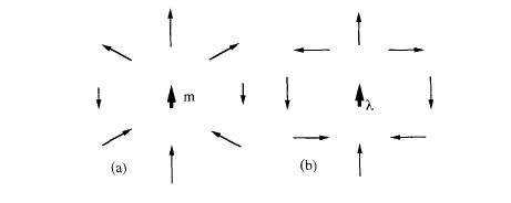
Figure 6.5. Comparison of the magnetic field produced by (a) a point dipole \(m\) and (b) a line dipole \(\lambda\).
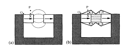
Figure 6.6. Flux leakage at an air - gap (a) contained by transversely magnetized cladding (b).
to the gap by magnetic cladding with radially magnetized ring magnets (Leupold 1996), as shown in figure 6.6(b). This is our first example of flux confinement by judiciously placed magnets which in this case point perpendicular to the desired field direction. The idea is to make the outer surface of the magnet an equipotential, so that there is no \(H\) field between any two points outside it. The magnetic potential difference \(\varphi_{\text{OP}}\) between a point \(O\) on the soft iron (which is itself a magnetic equipotential) and a point \(P(x,y)\) on the cladding must be zero, and it is given by the line integral along any path such as OXP. Thus \(\varphi_{\text{OP}}=H_{1}'x - H_{2}'y = 0\), hence \((B/\mu_{0}-M_{1})x + M_{2}y = 0\) if \(x\lt\ell\) and \((B/\mu_{0}-M_{1})\ell+H_{1}'(x - \ell)+M_{2}y = 0\) if \(x\gt\ell\). The suffixes 1 and 2 refer to the source magnet of length \(\ell\) and the cladding magnet, respectively. Since \(B\) is supposed to be parallel to OX in the source magnet there is no perpendicular component in the cladding magnet. This leads to the wedge - shaped cladding shown in the figure, with a half - angle \(\tan^{-1}[(B/\mu_{0}-M_{1})/M_{2}]\).
The same principle can be used to design long cylindrical magnets with no soft iron which generate a uniform longitudinal or transverse field in a hollow bore. In the transverse field design shown in figure 6.7(a), the outer surface will
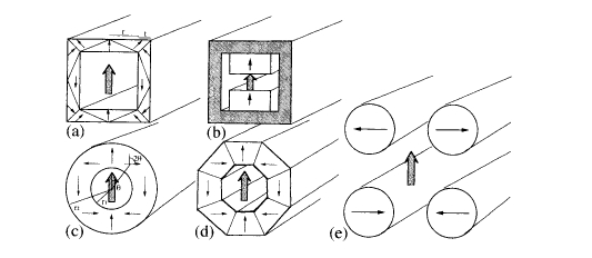
Figure 6.7. Designs for magnetic cylinders which produce a uniform transverse field.
be an equipotential provided \(t/r=\sqrt{2}-1\), in which case the field in the air - gap is \(0.293\ B_{r}\). Multiples of this field can be obtained by nesting similar structures one inside the other. Shimming the field to compensate for any imperfections in the magnets or assembly is achieved by placing appropriate compensating dipoles in the corners. The field in any long open magnetic cylinder will fall at the end to a value that is half that in the interior. The fall - off of field towards the end may be partly compensated by shimming or cladding at the ends to give a longer uniform - field volume.
An open cylinder (figure 6.7(a)) or a design with flat cuboid magnets and a soft - iron return path (figure 6.7(b)) may be used for nuclear magnetic resonance. NMR, especially the proton resonance, is an analytical tool increasingly used for quality control in the food and drug industries. The field must be shimmed to have the necessary high homogeneity of 1 part in \(10^{5}\). Nuclear magnetic resonance imaging (MRI) combines NMR with sophisticated signal processing to yield two - dimensional tomographic images of a solid object. It is widely used for non - invasive medical imaging. Radiofrequency radiation is absorbed at a frequency corresponding to the nuclear Zeeman splitting of a set of nuclei in the body. The distributions of spin - lattice and spin - spin relaxation times can be mapped and specific regions highlighted by means of magnetopharmaceutical agents. Proton images from \(^{1}\text{H}\) nuclei are generally obtained, but \(^{31}\text{P}\) and \(^{13}\text{C}\) are also feasible. Permanent - magnet flux sources supply fields of the order of \(0.3\ T\) in a whole - body scanner which are sufficient to provide adequate images. Although the fields are lower than those of competing superconducting solenoids, there is no need for any cryogenic installation. These systems are popular in Japan.
Figure 6.7(c) shows a different design where the direction of magnetization of any segment at angular position \(\theta\) in the cylinder is at \(2\theta\) from the vertical axis. According to (6.7), all segments now contribute to create a uniform field
across the air - gap in a vertical direction. Unlike the structure of figure 6.7(a), the inner and outer radii \(r_{1}\) and \(r_{2}\) can take any values without creating a stray field outside the cylinder. This ingenious device is variously known as a Halbach cylinder, a dipole ring or a 'magic cylinder'. The field in the air - gap is \[B_{0}=B_{\text{r}}\ln(r_{2}/r_{1})\] (6.8)
In practice, it is convenient to assemble the device from \(n\) trapezoidal segments, as illustrated in figure 6.7(d) for \(n = 8\). In this case, an extra factor \([\sin(2\pi/n)]/[(2\pi/n)]\) is included on the right - hand side of equation (6.8). In practice, the cylinders are never infinitely long; typical side length is comparable to the outer diameter, so the field is reduced by another factor \(f(z)\), where \(z\) is the distance from the centre. For example, the flux density at the centre of an octagonal cylinder with \(r_{1}=12\ \text{mm}\), \(r_{2}=40\ \text{mm}\) and length \(80\ \text{mm}\) made of a grade of Nd - Fe - B having \(B_{\text{r}} = 1.20\ T\) is \(1.25\ T\), compared to the value of \(1.44\ T\) calculated from (6.8).
There is no limit in principle to the magnitude of the field that can be produced in a Halbach cylinder, but in practice the coercivity and anisotropy field of the magnets limit the ultimate performance. Because of the logarithmic dependence in (6.8) and the high cost of rare - earth magnets, it becomes uneconomic to use permanent magnets to generate magnetic fields that exceed twice the remanence.
Another design, shown in figure 6.7(e), uses a few, typically four, six or eight, transversely magnetized rod - shaped magnets aligned around a central bore following the \(2\theta\) rule. These 'magnets' can be regarded as a further simplification of the configuration of figure 6.7(c) which affords access to the field from many different directions when a gap is left between the rods to let in a beam of radiation or even a microscope lens. Variable fields can be achieved by rotating the rods of the magnet, as discussed later in section 6.3.1. The field at the centre for \(n\) rods which are just touching is \[B=(n/2)B_{\text{r}}\sin^{2}(\pi/n)\] (6.9) Note that the value here is \(B = B_{\text{r}}\) for four rods with no gaps. In general, these cylindrical permanent magnet configurations deliver a field \(B = fB_{\text{r}}\), where \(f\) is a factor depending only on the relative dimensions of the magnet assembly.
Somewhat larger uniform fields can be produced at the centre of spherical or ellipsoidal structures, but channels must be cut to provide access to the air - gap at the centre. The largest field that has been generated with permanent magnets is \(4.5\ T\) in a region of diameter \(2\ \text{mm}\) at the centre of a spheroidal magnet mass \(8\ \text{kg}\) (Cugat 1998).
Non-Uniform Magnetic Fields: Behavior, Challenges, and Practical Usess
Inhomogeneous fields are useful for particle beam control, focusing in cathode ray tubes and other electron - optic machines, generating microwaves and other

Figure 6.8. Some cylindrical magnet structures which produce inhomogeneous fields: (a) a quadrupole field, (b) a hexapole field and (c) a uniform field gradient.
Magnetic recording involves a pattern of spatially varying magnetization in a medium which is usually detected via its non - uniform stray field.
The cylindrical configurations in figure 6.7 may be modified to generate various sorts of inhomogeneous field, particularly useful for beam control. Halbach's original cylindrical magnets were used to produce a quadrupole field for focusing beams of charged particles. Higher multipole fields than the dipole field are obtained by having the orientation of the magnets in the ring vary as \((v/2)+1\), where \(v = 2\) for a dipole field, \(v = 4\) for a quadrupole field and so on. The field at the centre of the quadrupole is zero, but whenever the beam deviates it experiences a force in an increasing field which causes its trajectory to curve back to the centre. Figure 6.8(a) shows an ideal quadrupole source. A practical hexapole as in figure 6.8(b) is used to produce ions from a plasma contained in a magnetic bottle.
Axially magnetized rings with a central return path known as'magnetrons' are used in sputtering systems to increase the ionization of the plasma near the target by altering the paths of the electrons in helices around the field lines. The magnets in an ion pump have a similar function.
Shown in figure 6.8(c) is an arrangement of four rods which produces a uniform magnetic field gradient in the vertical direction in the space at the centre. Field gradients are most useful for exerting forces on magnets. Although it is impossible to design a field configuration which will draw a small magnet towards a fixed point in space, there are circumstances when stable levitation of a permanent magnet at a point is possible; these involve either spinning the magnet, active feedback with electric current controlling the forces along one axis or the use of a superconductor where supercurrents flow in response to the magnet's position.
Note that a sheet of superconductor provides a direct image of a permanent magnet, whereas a sheet of soft iron provides an inverted image (figure 6.9). Superconductors are unavailable for use at room temperature, but iron mirrors
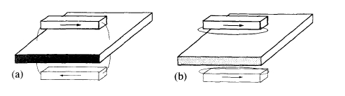
Figure 6.9. Images of a permanent magnet in a sheet of (a) soft iron or (b) superconductor.
may be employed to simplify the design of some permanent - magnet circuits. The configuration of figure 6.7(e), for example, can be reduced to just two magnets with a horizontal iron sheet passing through the centre (figure 6.15(c)). While \(\partial B/\partial x,\partial B/\partial y>0,\partial B/\partial z < 0\) can be used to levitate a diamagnetic material, provided the product \(\partial B_{x}/\partial x...\) are sufficiently great. Such a point exists on the axis of a vertical solenoid. Magnetic levitation is discussed further in section 6.3.
The arrangement of figure 6.7(e) can be modified to create a field gradient along its axis if the directions of magnetization of alternate rods twist uniformly clockwise or anticlockwise along their length. Another type of permanent - magnet structure creates an inhomogeneous magnetic field along the axis of the magnet, which is the direction of motion of a charged particle beam. Microwave power tubes such as the travelling wave tube are designed to keep the electrons moving in a narrow beam over the length of the tube and focus them at the end while coupling energy from an external helical coil. Originally this was achieved by applying a uniform axial field from a resistive solenoid, but the design with permanent - magnet focusing by a periodic axial field in figure 6.10 is just as effective, and represents a great saving in weight and power when SmCo5 magnets are used. Other microwave devices employing permanent magnets include klystrons and'magnetron' sources, including those with ferrite magnets produced in large quantities for domestic microwave ovens. The cyclotron frequency of an electron in a field \(B\) is \[f_{\text{c}}=\frac{eB}{2\pi m_{\text{e}}}\] (6.10) or \(28\ \text{GHz}\ T^{-1}\). The field in a domestic microwave magnetron is about \(0.1\ T\), giving \(3\ \text{GHz}\) radiation with wavelength \(\lambda\approx10\ \text{cm}\).
In a synchrotron, electrons with relativistic velocities \(v\approx c\) are guided by bending magnets around a closed track which may be tens or hundreds of metres in diameter (figure 4.2). Insertion devices are permanent - magnet structures located in straight sections of the track. They serve to generate intense beams of polarized hard radiation (UV and x - ray) from the energetic electrons
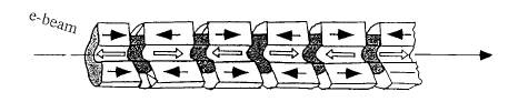
Figure 6.10. A microwave travelling wave tube with a periodic axial field.
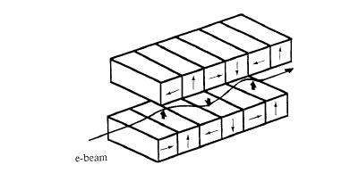
Figure 6.11. A wiggler magnet used to generate intense electromagnetic radiation from an electron beam.
beam by setting up a sinusoidal transverse field of wavelength \(\Lambda\). These devices are generically known as wigglers, since they cause the electrons to travel in a sinuous path. Similar structures are used in free - electron lasers. A wiggler design which includes segments magnetized in a direction parallel to the electron beam to concentrate the flux is shown in figure 6.11. As the electrons traverse the insertion devices, they radiate at a frequency \(c/\Lambda\). When the frequency of oscillation in the insertion device exceeds the cyclotron frequency, the radiation is coherent and the insertion device is then known as an undulator. From (6.10), the condition for coherent radiation is \(B\Lambda<2\pi m_{\text{e}}c/e = 1.07\ T\ cm\). The intensity of the radiation from a wiggler varies as \(2N\) where \(N\) is the number of magnet periods, but the intensity from an undulator varies as \(N^{2}\). The radiation is linearly polarized perpendicular to the field. Circularly polarized radiation can be obtained by using two devices producing horizontal and vertical sinusoidal fields with a relative phase shift of \(\pi/2\). The European Synchrotron Radiation Facility in Grenoble, for example, has 150 m of insertion devices, using several tons of \(\text{Nd}_{2}\text{Fe}_{14}\text{B}\) magnets.
Magnetic Separation
Magnetic separation (Gerber 1994) is a technology based on inhomogeneous or time - varying magnetic fields which affords unsung economic and social benefits
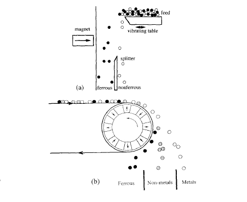
Figure 6.12. (a) Open - gradient magnetic separation and (b) electromagnetic separation with permanent magnets.
from the tiphead to the haematology laboratory. The forces involved can be expressed in terms of an energy gradient. The expression for the energy of a pre - existing magnetic moment \(\boldsymbol{m}\) in a field \(\boldsymbol{H}\) is \(-\mu_{0}\boldsymbol{m}\cdot\boldsymbol{H}\), leading to the expression \[\boldsymbol{F}=\mu_{0}\nabla(\boldsymbol{m}\cdot\boldsymbol{H})\] (1.14) However, when a small moment \(\boldsymbol{m}=\chi V\boldsymbol{H}\) is induced by the field in a material of volume \(V\) and susceptibility \(\chi\), the expression becomes \[\boldsymbol{F}=(1/2)\mu_{0}\chi V\nabla(H^{2})\] (6.11)
To separate ferrous and non - ferrous scrap or to select minerals from crushed ore on the basis of their magnetic susceptibility, it is sufficient to use open - gradient magnetic separation. Here material tumbles through a region where there is a strong magnetic field gradient, as shown in figure 6.12(a). Early patents on magnetic separation of iron ore date from 1792. The field gradient may be produced by permanent magnets or electromagnets. Material with the greatest susceptibility will be deflected most. Since the force is proportional
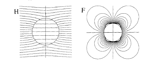
Figure 6.13. Field and force patterns around a cylindrical iron wire in a high - gradient magnetic separator.
to the particle volume (mass), the trajectory is independent of particle size and separation is susceptibility selective. Field gradients in open - gradient magnetic separators may be of the order of \(100\ T\ m^{-1}\) and separation forces are of the order of \(10^{8}\ N\ m^{-3}\).
Because of the ubiquity of ferrous scrap, permanent - magnet traps are commonly used to remove it in industrial processes such as milling of foodgrains. A specialized form of open - gradient separation is provided by the cow magnet. Valuable ruminants are forced to swallow a teflon - coated magnet which resides in one of their stomachs, where it captures nails and fragments of barbed wire which would harm the beast if allowed to proceed through its digestive tract—a good example of a technological fix to a problem created by technology!
High - gradient magnetic separation is a method suitable for capturing weakly paramagnetic material such as red blood cells. Here a liquid containing the paramagnetic solids in suspension passes through a tube filled with a fine ferromagnetic steel mesh or steel wool. When a uniform external field is applied, the fine wire (about \(50\ \mu m\) in diameter) distorts the flux pattern, creating local field gradients as high as \(10^{5}\ T\ m^{-1}\) and separation forces can reach \(10^{11}\ N\ m^{-3}\). Figure 6.13 shows the field and force patterns around such a wire. The paramagnetic material remains stuck to the wires until the external field is switched off, when it may be flushed out of the system. Electromagnets or switchable permanent magnets are used to create the field.
A different principle is employed in electromagnetic separation to sort non - ferrous metal such as aluminium cans from non - metallic material in a stream of refuse. A fast - moving conveyor belt carries the rubbish over a static or rotating drum with embedded permanent magnets. The relative velocity of the magnets and the refuse may be as high as \(50\ m\ s^{-1}\). Eddy currents induced in the metal create a repulsive field, and the metal is thrown off the end of the belt in a different direction to the non - metallic waste (figure 6.12(b)). In electromagnetic separation, deflection depends on the ratio of conductivity to Density, so it is possible to separate different metals such as aluminium, brass and copper. The first patent on eddy - current separation was secured by Thomas Edison himself. Other force applications of permanent magnets which involve mechanical recoil are discussed in section 6.3.
Magnetic Recording
Digital and analogue recording (Kryder 1992) is a huge industry, consuming vast quantities of ferrite and other semi - hard magnetic materials for recording media (figure 1.15), and using sophisticated miniature magnetic circuits in the read and write heads. The media consist of thin films or dispersions of single - domain particles in a polymer matrix, with an easy direction of magnetization parallel to the substrate. Materials commonly used for particulate media on tapes and floppy disks are acicular \(\gamma\)-\(Fe_{2}O_{3}\) (especially with Co surface doping), \(\text{CrO}_{2}\) and iron metal, whereas Co - Cr alloys are generally used for the thin - film media on hard disks (section 5.2.1.2). The recorded information is normally erasable so the media must be reusable. Emphasis in magnetic recording is therefore on controlling nucleation of reverse domains, whereas in permanent magnetism the emphasis is on avoiding nucleation. Nevertheless, as recording densities increase, there is a trend to materials with ever - higher coercivities, \(\mu_{0}H_{\text{c}}>0.3\ T\), so that permanent - magnet materials like \(\text{BaFe}_{12}\text{O}_{19}\) or even PtFe or \(\text{SmCo}_{5}\) might be considered as recording media in the future. Perpendicular recording may also help to improve density. Certain magnetic records like those on credit or identity cards are not intended to be erased. A brief discussion of some aspects of magnetic recording is given here. An extended treatment can be found in Bertram (1994), and other texts include White (1984), Sellmeyer and Shan (1997) and Kryder (1994).
Digital information is encoded in the direction of magnetization of domains located at identifiable points on tracks in the magnetic medium (figure 6.14). Perpendicular recording allows higher record densities, but it requires sufficiently strong uniaxial anisotropy in a direction perpendicular to the plane of the medium so that the anisotropy field exceeds the demagnetizing field, \(2K_{1}/\mu_{0}M_{\text{s}}>M_{\text{s}}\), a weaker condition than that for a true permanent magnet, where \(K_{1}>\mu_{0}M_{\text{s}}^{2}\) (1.26). In both cases, a square hysteresis loop is desirable.
Recording is carried out by applying a field which is locally sufficient to switch the magnetization. Normally this is done with a current pulse in an inductive write head. Williams and Comstock (1972) developed a model for the recording process which predicts the width \(a\) of the recorded transition in a material with a square hysteresis loop to be \[a = \sqrt{\frac{M_{\text{r}}\delta d}{\pi H_{\text{c}}}}\] (6.12) where \(\delta\) is the medium thickness and \(d\) is the head - medium spacing. Hence the
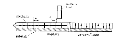
>Figure 6.14. A schematic of in - plane and perpendicular magnetic recording. The inset shows the detail of a thin - film magnetoresistive head with a permanent magnet bias layer.
need to reduce these distances and increase coercivity for the highest recording densities. In hard - disk drives, the head - medium separation is 20 - 100 nm. The write head consists of a flat coil sandwiched between films of a soft material such as permalloy, \(\text{Fe}_{23}\text{Co}_{64}\text{Ni}_{12}\) or \(\text{Fe}_{94}\text{Ta}_{3}\text{N}_{3}\) which form the poles of a miniature electromagnet. The written bits are narrow bands oriented across the track, which are magnetized by the stray field at the edges of the two flat poles.
The direction of magnetization of the medium may be read via the stray field measured close to the surface using an inductive read head or a thin - film magnetoresistance sensor made of permalloy. Magnetoresistive multilayers or spin - valve structures are used for the highest densities (about 16 bits \(\mu m^{-2}\); 10 Gbits/inch2). These sensors are illustrated in section 6.5.2. Some read heads include a hard - magnetic layer of \(\text{Co}-\text{Cr}\) or \(\text{Co}-\text{Pt}\) to bias the sensor layer, while other designs depend on exchange bias from an adjacent layer of an antiferromagnet such as NiO, FeMn or IrMn, or the stray field produced by a soft adjacent layer which is magnetized in the sense current in the magnetoresistive layer. A small bias field is needed on a magnetoresistive read head so that it can operate in a linear region of high reversible sensitivity \(dR/dH\) (R is the film resistance) as the stray field \(H\) changes sign. Permanent - magnet films also serve to stabilize the domain structures in read and write heads.
Thermomagnetic recording is an alternative method where the medium is heated locally by a pulsed laser to a temperature where the coercivity is small, and then cooled in a weak bias field. This is combined with stray - field reading or magneto - optic reading based on the Kerr effect (section 4.2.4.2)—the plane of polarization of a reflected beam from a semiconductor diode laser is rotated by an angle \(\pm\theta_{\text{K}}\) on reflection from a \(\uparrow\) or \(\downarrow\) domain; \(\theta_{\text{K}}\) is large. Suitable magneto - optic media are amorphous \(\text{R}_{100 - x}\text{T}_{x}\) films, where R is a rare earth such as terbium and T is a transition metal such as cobalt. The rare earth has a substantial Kerr effect on account of its strong spin - orbit coupling. During recording the medium is heated above the Curie point or above the compensation point, which is near room temperature when \(x\approx0.7\) in this system. Use of an amorphous medium eliminates grain - boundary noise.
Strictly speaking, 'thin - film permanent magnet' is an oxymoron. A uniformly magnetized thin film creates no flux whatsoever in the surrounding air. The perpendicular component of magnetization \(M_{\perp}\) creates a demagnetizing field \(H_{\text{dm}}=-D_{\perp}M_{\perp}\) where \(D_{\perp}=1\). Hence, \(B_{\perp}=\mu_{0}(H_{\text{dm}} + M_{\perp}) = 0\) inside the magnet and also outside it, by continuity. Likewise the parallel component \(B_{\parallel}\) is zero by Ampere's theorem, since \(H_{\parallel}=-D_{\parallel}M_{\parallel}=0\) because \(D_{\parallel}=0\). Useful flux outside a film only arises when it is patterned, lithographically or magnetically, on the scale of the film thickness. Hence, the bit size in thin - film media is typically no more than an order of magnitude greater than the film thickness, and the in - plane dimensions of thin - film magnets used to create bias fields are no more than an order of magnitude greater than their thickness, so that \(D_{\parallel}\approx0.1\).
Ultrahigh - density magnetic recording involves recording a bit on the magnetization of a group of \(N\) single - domain grains in a thin film. For a good signal - to - noise ratio, the individual grains should be magnetically decoupled. The signal - to - noise ratio in dB is then of the order of \(10\log N\); a value of about 30 dB is required which means that \(N\) is of the order of 1000. The smallest grain size is determined by the condition that superparamagnetic fluctuations of the grains' magnetization must not be excited thermally. The highest recorded densities will therefore be found for magnetic media made from materials with the highest possible anisotropy. In the case of \(\text{SmCo}_{5}\), \(K_{1}=17.2\ \text{MJ}\ m^{-3}\) (table 5.11) and the condition for superparamagnetic blocking at room temperature of a particle of volume \(V\), \(K_{1}V/k_{\text{B}}T>25\) (section 3.4.3.2), implies a particle size of a few nanometres. If the film thickness is 10 nm, then the bit size would be \(600\ nm^{2}\), leading to ultimate densities of the order of 1000 bits \(\mu m^{-2}\) [645 Gbits/inch2]. Even higher densities will demand patterned media where small particles in determined positions along a track are individually addressed.


