Basis of Permanent Magnetism: A Comprehensive Guide to Magnetic Moments, Magnetization, and Hysteresis

Basis of Permanent Magnetism is one of the most intriguing phenomena in the field of solid-state physics and materials science. Its foundation lies in the magnetic moments of unpaired electrons in magnetically ordered solids. These magnetic moments, when aligned through exchange interactions, give rise to a net magnetization, creating a persistent magnetic field that remains stable below the Curie point. This remarkable phenomenon has profound implications in both fundamental science and practical applications.These moments, when coupled via exchange interactions, give rise to a net magnetization at temperatures below the Curie point. This magnetization produces a magnetic field that is nonlinear and often irreversible under the influence of an external magnetic field, leading to the formation of hysteresis loops.

In this detailed guide, we’ll delve into the basis of permanent magnetism, covering everything from atomic magnetic moments and magnetization to hysteresis loops and the practical applications of permanent magnets. Additionally, we’ll explore how magnetic fields interact and the challenges and advancements in this field.

Basis of permanent magnetism

Magnetically ordered solids have atomic magnetic moments due to unpaired electrons. The atomic moments are coupled by exchange interactions which may give a net magnetization at all temperatures below the Curie point. Magnetization creates a magnetic field, and is itself a nonlinear and irreversible function of an externally applied field, represented on the hysteresis loop. Hysteresis depends both on the microstructure of the material and its magnetic anisotropy. These ideas are developed in this introductory section.

Understanding Magnetic Moments

The fundamental building block of permanent magnetism is the magnetic dipole moment of electrons. Every electron in an atom contributes to the overall magnetic moment through:

Spin Motion: The intrinsic angular momentum of electrons.
Orbital Motion: The movement of electrons around the nucleus.

The total magnetic moment of a material is the sum of the individual moments of its electrons. However, only unpaired electrons contribute to net magnetization because their moments do not cancel out.

Why Nuclear Moments Are Negligible:

Nuclear magnetic moments are approximately 1,000 times weaker than electronic moments, making their contribution to a material’s overall magnetism negligible.

Magnetization and Magnetic Fields:

Magnetization (M) refers to the magnetic moment per unit volume of a material. It measures the intensity of the magnetic field generated by the material and is expressed in amperes per meter (A/m).

External vs. Internal Magnetic Fields:

External Field (H):
This is the magnetic field applied to the material, such as the field generated by a solenoid.
Internal Field (H’):
Inside the material, the total field is a combination of the external field and the field generated by the magnetized material itself.

The internal field is influenced by the demagnetizing field (Hdm), which arises due to the magnet’s geometry and causes the internal field to oppose the magnetization.

Hysteresis Loops:

The relationship between magnetization (M) and the applied field (H) is nonlinear and exhibits hysteresis. The hysteresis loop is characterized by:

Remanence (Mr): The residual magnetization when the external field is removed.
Coercivity (Hc): The reverse field required to demagnetize the material.

Hysteresis loops are critical for understanding permanent magnetism and are widely used in the design of magnetic devices.

Moments, magnetization and magnetic fields

Magnetic moment:

The key concept in solid-state magnetism is the magnetic dipole moment m. Almost all the moments that concern us are associated with atomic electrons, which are the elementary magnets in solids. The dipole moment of a magnet is the sum of the dipole moments of all its constituent electrons. The magnetic moment per unit volume is the magnetization, M. Nuclear moments are a thousand times smaller than electronic moments, and their contribution to the magnetization is negligible.

Since 1820, when Oersted demonstrated the equivalence of the effects produced by magnets and circulating electric currents, the relation between electricity and magnetism has been secure. A small current loop is equivalent to a magnetic moment

$$m = I\mathcal{A} \quad (1.1)$$

where I is the circulating current and A the area of the loop. Electrons carry an electric charge -e = -1.602×10^-19 C in perpetual motion according to the laws of quantum mechanics, so they behave as elementary current loops. Magnetic phenomena can be interpreted as arising from electric current althougha difficulty arises with electronic spin (problem 1.4). The deep connection between electricity and magnetism is manifest in the SI unit system, where m is expressed in A m2 . No magnetic analogue of the electric charge is known, despite great efforts to discover a magnetic monopole. Nevertheless, it will be helpful to introduce fictitious magnetic surface charges to simplify certain calculations.

Magnetization and magnetic field

A homogeneously magnetized solid is characterized in the continuum approximation by its magnetization M(r) = δm / δV, where δV is a volume element of the magnet. Units of M are A m^-1. These are the same as the units of the magnetic field H created in free space by a magnet or by an electric current. For instance, the field inside a long solenoid with n turns per metre carrying a current I is H = nI. The H field is sometimes called the'magnetizing force' since the magnetic or superconducting state of a solid is a response to this field. The relation between the locally varying quantities M and H, known as the magnetic equation of state, is nonlinear, multivalued and dependent on the size, shape and history of the magnet. The function M(H) is known as the hysteresis loop (figure 1.1); it is characterized by its intercepts M_r (remanence) and H_c (coercivity). The hysteresis loop is the central datum of permanent magnetism; physicists want to understand it, materials scientists want to improve it and engineers want to exploit it in useful applications.

It is important to distinguish the externally applied magnetic field H that exists in the absence of any magnetized material from the total, internal magnetic field H' = H + H_dm. Here the demagnetizing field

$$H_{dm}(r) = -\frac{1}{4\pi} \int \frac{(r - r')\nabla \cdot M(r') dr'}{|r - r'|^3} \quad (1.2)$$

is created by the magnet; outside the magnet it is also known as the stray field. The demagnetizing field H_dm is closely related to the dipole field H_d created by the atomic magnetization distribution M(r) at any point. The magnetic field created at r by a point dipole M is

$$H_d = \frac{1}{4\pi}[3r(r\cdot m)/r^3 - m/r^3] \quad (1.3)$$

hence

$$H_d = \frac{1}{4\pi} \int \frac{3(r - r')(r - r') \cdot M(r') - |r - r'|^2 M(r')}{|r - r'|^5} dr' \quad (1.4)$$

Inside the magnet, these quantities differ by the Lorentz field H_L = M/3, so that H_d = H_dm + H_L (section 2.1.7.3); outside the magnet they are identical.

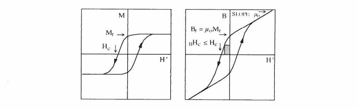
Figure 1.1. Typical hysteresis loops for a permanent magnet. The M(H) and B(H) loops are obtained after saturating the magnetization. The two loops are related by equation (1.3). The shaded area indicates the maximum energy product (BH)_max.

The divergenceless field B, known as flux density or induction, is defined by

$$B = \mu_0(H' + M). \quad (1.5)$$

Here μ₀ = 4π × 10^-7 N A^-2 is the magnetic constant known as the permeability of free space which is involved whenever the H field interacts to exert a force on a magnet or a current-carrying conductor.

Like M, the fields H' and B may vary on a local scale. They obey the magnetostatic field equations which are obtained from Maxwell's equations by neglecting free currents:

$$curl\ H' = 0 \quad and \quad div\ B = 0. \quad (1.6a, b)$$

In free space, M = 0 and B₀ = μ₀H', but generally the vector character of (1.3) and the nonlinear dependence of M on H' mean that inside the material B and H' are neither parallel nor proportional (figure 1.2). The unit of B is V s m^-2 = N (A m)^-1, which is given a special name, the tesla (T). The magnitude of the tesla is convenient for discussing ferromagnetism, and we will often multiply H and M by μ₀, and express the results in tesla instead of A m^-1. The quantity μ₀M is given the symbol J by engineers, who call it the polarization, so that (1.5) may be written as B = μ₀H' + J. The remanent polarization of a good permanent magnet is usually about 1 T [10 kG], although that of ferrites does not exceed 0.6 T [6 kG]. The magnetization of pure iron is 1.76 MA m^-1 [1760 emu cc^-1], corresponding to a polarization of 2.15 T [21.5 kG] .

A typical electrotechnical application of permanent magnets requires a uniform magnetic flux density B of order 1 T. The purpose of the magnet is to deliver flux into an airgap. By comparison, iron-core electromagnets and superconducting magnets typically produce flux densities of up to 2 T and 15 T, respectively. Current pulses in coils can create fields of more than 100 T for some tens of microseconds. At the other end of the scale, the stray fields

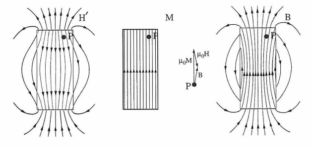
Figure 1.2. Magnetic field H' and flux density B due to a uniformly-magnetized bar-shaped permanent magnet of magnetization M. Relation (1.5) is illustrated at point P.

detected in magnetic recording are of order 10 mT, the geomagnetic field is about 50 μT and fields of order 1 nT are generated by electric currents in the brain. Other applications exploit the fact that permanent magnets are able to attract magnetized materials. The maximum force obtainable is F = μ₀M²A/2, where A is the cross-sectional area of the magnet. Taking μ₀M = 1 T, F/A is 400 kN m^-2, equivalent to about 4 kg cm^-2.

Dipolar fields and domain formation

Consider a piece of magnetized material subject to no externally applied field, so that the field H' entering (1.6a) equals H_dm. For a uniformly magnetized bar the quantities M, H' and B are shown in figure 1.2. It may be seen that the magnetic field H' produced by the magnet is oppositely directed to M in the volume of the magnet. In other words, the magnet produces its own demagnetizing field. As a consequence, the uniformly magnetized state of macroscopic magnets is at best metastable. Lower-energy states exist where the magnetization is broken up into domains magnetized in different directions so that the solid as a whole has no net magnetization. In a macroscopic sample where we can average the magnetization over a scale which is large compared with the domain size, M is regarded as the average magnetization of the sample rather than the local magnetization in a domain. The magnetization shown in the M(H') hysteresis loop of figure 1.1 is such a domain average.

The local, spontaneous magnetization of iron is greater than that of any commercial permanent magnet, but the demagnetizing field makes it impossible to retain the fully magnetized state which usually breaks up into domains. Much of the art of making magnets consists in realizing a suitable shape or microstructure which will allow a metastable, highly magnetized state to persist after saturating.

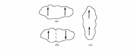
Figure 1.3. Sketches of homogeneous and inhomogeneous magnetization states. (a) is magnetostatically much less favourable than the multidomain configuration (b) and would have to be maintained by strong uniaxial anisotropy. The prolate configuration (c) is comparatively stable and needs less anisotropy to remain permanently magnetized.

the magnetization in an external field. In earlier times, the only way to achieve this was by reducing the demagnetizing field by means of elongated needle, bar and horseshoe shapes (figure 1.3). Such magnets have been obsolete for 50 years; they can still be seen in museums and primary school science texts.

Magnetostatic energy and demagnetizing fields

From the units of $M$, $H$ and $B$ it follows that expressions such as $\mu_{0}M H V$, $B H V$ and $B M V$ are energies, where $V$ is the magnet volume. It also follows that alternative units for the magnetic moment $m$ and magnetization $M$ are $J T^{-1}$ and $J (T m^{3})^{-1}$. In particular, a way to define the magnetostatic self-energy of a permanent magnet is

\[E_{ms} = -\frac{\mu_{0}}{2} \int M \cdot H_{dm} d r.\] (1.7)

Here the integral is restricted to the volume of the magnet, as $M$ vanishes outside. Essentially, this energy represents the mutual magnetostatic interaction of the elementary dipoles of which the magnet is composed. To extract information from (1.7) we exploit the identity $\int B \cdot H_{dm} dV = 0$. This identity, where the integral is over all space, both inside (i) and outside (a) the magnet, is valid in the absence of conduction currents¹. Hence, from (1.5),

\[\int_{i} M \cdot H_{dm} d r + \int_{i} H_{dm}^{2} d r + \int_{a} H_{dm}^{2} d r = 0.\] (1.8)

From (1.7) and (1.8) the magnetostatic self-energy can also be written as $E_{ms} = (\mu_{0} / 2) \int H_{dm}^{2} d r$, where the integral now extends over all space.

¹ The proof is straightforward. Using $B = curl A$, where $A$ is the vector potential, $H_{dm} = -\nabla \varphi_{m}$, where $\varphi_{m}$ is the scalar potential, and $curl (\nabla \varphi_{m}) = 0$, one obtains the condition $\int \nabla \cdot (A \times H_{dm}) d r = 0$, which is equivalent to $\int A \times H_{dm} dS = 0$. Both $A \propto 1 / r^{2}$ and $H_{dm} \propto 1 / r^{3}$ fall off rapidly with distance, so that the surface integral of $A \times H_{dm}$ is zero if it is extended to infinity.

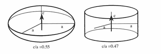
Figure 1.4. Optimally shaped ellipsoidal magnet with D = 1 /2 ( left ), and an equivalent cylinder with nearly uniform magnetization ( right).
Only in a few cases is it easy to determine $E_{ms}$. For instance, in uniformly-magnetized ellipsoids $H_{dm}$ is also uniform. If the magnetization lies along a major axis,

\[H_{dm} = -DM\] (1.9)

so then $E_{ms} = \mu_{0}D M^{2}V/2$. The quantity $D$, known as the demagnetizing factor, obeys the inequality $0 \leq D \leq 1$. It turns out that $D \approx 0$ for elongated needle shapes, $D = 1/3$ for spheres and $D \approx 1$ for plate-like magnets (section 2.1.7). In practice, shapes like cylinders can be assimilated to ellipsoids since the demagnetizing field is uniform over most of their volume (figure 1.4).

The magnetostatic energy $E_{ms}$ contains contributions from both inside and outside the magnet, but it is the energy $E' = (\mu_{0}/2) \int_{a} H_{dm}^{2} dV$ stored in the field outside the magnet that is of more interest, since only this part is available for practical uses.

From (1.5) and (1.8) we deduce

\[E' = -\frac{1}{2} \int_{i} B \cdot H_{dm} dV.\] (1.10)

Using (1.9) and assuming $M$ is a uniform, macroscopically averaged magnetization independent of $H_{dm}$, we obtain $E' = (1/2)\mu_{0}D(1 - D)M^{2}$ for ellipsoids. This energy is maximized for $D = 1/2$, which corresponds to the slightly oblate shape shown in figure 1.4. The energy product for a uniformly magnetized macroscopic magnet is defined as the product $-B \cdot H_{dm}$, which is equal to $2E'/V$. It is specified empirically by the shape of the second quadrant of the $B-H'$ loop in figure 1.1. The maximum energy product $(BH)_{max}$ is shown by the shaded area in the figure. When $D = 1/2$, the theoretical $(BH)_{max}$ is $\mu_{0}M^{2}/4$. In practice, the magnetization decreases with increasing demagnetizing field, so that the maximum energy product is obtained for demagnetizing factors $D < 1/2$. The energy product of carbon-steel magnets is of the order of $1 kJ m^{-3}$, whereas that of modern rare-earth permanent magnets exceeds $200 kJ m^{-3}$. Compared to other energy-storage media such as fuel, permanent magnets store tiny amounts of energy, but the great advantage is that this energy is available in a remarkably useful form.

Let us now consider the effect of an externally applied field $H$ on a small magnet of variable magnetization. There is an additional term in the magnetostatic energy

\[E_{Z} = -\mu_{0} \int M \cdot H \,dV\] (1.11)

called the Zeeman energy which describes the interaction of the magnet with the external field. It should be noted that the expressions for the self-energy (1.7) and Zeeman energy (1.11) differ by a factor 1/2 (section 2.1.7).

When $M$ is constant throughout the magnet and the field is uniform over its volume, the Zeeman energy becomes

\[E_{Z} = -\mu_{0}m \cdot H\] (1.12)

where $m = MV$. Differentiating this equation gives important expressions for the torque

\[\Gamma = \mu_{0}m \times H\] (1.13)

and the force

\[F = \mu_{0}\nabla(m \cdot H)\] (1.14)

exerted on a magnet by an external field. There is no force when a magnet is aligned with a uniform magnetic field.

FAQ
Q: What is the basis of permanent magnetism?
The basis of permanent magnetism lies in atomic magnetic moments created by unpaired electrons. These moments align via exchange interactions to produce net magnetization below the Curie temperature.
Q: What is a hysteresis loop?
A hysteresis loop shows the relationship between magnetization and an applied magnetic field, highlighting properties like remanence and coercivity.
Q: What factors affect the performance of permanent magnets?
Factors include temperature, magnetic anisotropy, material composition, and the presence of demagnetizing fields.
Q: What are some common applications of permanent magnets?
Permanent magnets are used in motors, data storage, medical imaging, consumer electronics, and magnetic levitation systems.
Summary
The basis of permanent magnetism lies in the collective alignment of atomic magnetic moments, driven by exchange interactions. Key concepts such as magnetization, hysteresis loops, and demagnetizing fields are critical for understanding how permanent magnets work and how they can be optimized for various applications.
From powering electric motors to enabling magnetic resonance imaging, permanent magnets are integral to modern technology. As advancements in materials science continue, the potential of permanent magnetism remains limitless.