
3.2 Basic Micromagnetics: Principles and Applications
A central problem in solid-state magnetism is to relate field-dependent magnetization configurations \(M(\mathbf{r})\) to atomic parameters such as \(M_{\text{s}}\) and \(K_{1}\). This subject is called micromagnetics. It concerns not only magnetic domains and domain walls but also with problems such as the onset of magnetization reversal (nucleation) and the rotation of the magnetization of misaligned grains. Many micromagnetic results apply to both hard and soft magnets, but the dominance of the magnetocrystalline anisotropy in permanent magnets leads to a number of characteristic features.
A major difficulty is the treatment of the magnetostatic self-interaction. Consider, for example, the effect of demagnetizing fields in homogeneous
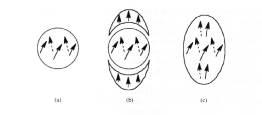
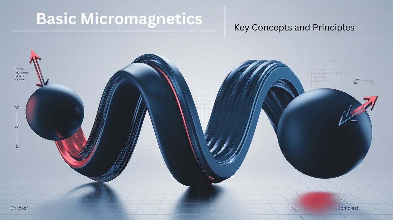
Figure 3.11. Magnetostatic interactions in homogeneous particles. The difference between spheres (a ) and prolate ellipsoids (c) cannot be reduced to a demagnetizing-field contribution caused by fictitious pole caps (b).
ellipsoids of revolution (figure 3.11). In the demagnetizing-field approximation, the prolate ellipsoid differs from the sphere by having a somewhat smaller demagnetizing field (figure 3.11(b)), that is the shape anisotropies are different. However, this is not the only consideration. First, the magnetization must be continuous throughout the magnet, which modifies the exchange and anisotropy energy densities (figure 3.11(c)). Second, the three spin configurations shown in figure 3.11 exhibit closed flux-line contributions in the planes \(z = \) constant. These contributions are energetically favourable and we will see that they dominate the onset of magnetic reversal in homogeneous particles having radii larger than about 10 nm.
The Micromagnetic Energy Functional: A Core Concept in Magnetism
In micromagnetics, it is common to start from energy functionals such as (1.30). The most general form used in this chapter is
\(E = E_{\text{ex}} + E_{\text{Z}} + E_{\text{dm}} + E_{\text{a}}\) (3.52)
where
\(E_{\text{ex}} = \int A\left(\nabla\frac{\mathbf{M}}{M_{\text{s}}}\right)^{2} \text{d}V\) (3.53)
is the exchange energy (section 3.2.1.1),
\(E_{\text{Z}} + E_{\text{dm}} = -\mu_{0} \int \left(\mathbf{M} \cdot \mathbf{H} + \frac{1}{2}\mathbf{M} \cdot \mathbf{H}_{\text{dm}}(\mathbf{M})\right) \text{d}\mathbf{r}\) (3.54)
are the magnetostatic interactions discussed in sections 2.1.4.1 and 2.1.7.1, and
\(E_{\text{a}} = \int \left\{(K_{1} + 2K_{2})\frac{(\mathbf{n} \cdot \mathbf{M})^{2}}{M_{\text{s}}^{2}} - K_{2}\frac{(\mathbf{n} \cdot \mathbf{M})^{4}}{M_{\text{s}}^{4}}\right\} \text{d}\mathbf{r}\) (3.55)
is the anisotropy energy (section 3.1). Here \(n\) denotes the unit vector of the local anisotropy direction and \(A\) is the exchange stiffness penalizing deviations from the homogeneous magnetization state. In (3.55) we have restricted ourselves to the leading uniaxial anisotropy constants \(K_{1}\) and \(K_{2}\), which is a good approximation in many cases (compare section 3.1.1). The parameters entering (3.53)–(3.55) are assumed to be known in general and \(A\), \(K_{1}\), \(K_{2}\), \(M_{\text{s}}\) and \(n\) are functions of \(r\), so that these equations apply to both homogenous and inhomogenous materials.
The description of the magnetostatic self-interaction is particularly complicated. Maxwell's equations yield a continuum field \(H' = H + H_{\text{dm}}\) (sections 1.1.1.2 and 2.1.1.2) which must be distinguished from the atomic field \(H_{\text{at}} = H + H_{\text{d}} = H + H_{\text{dm}} + M/3\) (section 2.1.7.3). Fortunately, this difference is of minor importance for the determination of \(M(\mathbf{r})\), because the difference between the associated magnetostatic energies \(E_{\text{dm}}\) and \(E^{*}\) (section 2.1.7) is a constant. We can therefore replace (3.54) by
\(E_{\text{Z}} + E^{*} = -\mu_{0} \int M \cdot H \text{d}V - \frac{\mu_{0}}{2} \int M(\mathbf{r}) \cdot \mathcal{G}(\mathbf{r} - \mathbf{r}') \cdot M(\mathbf{r}') \text{d}\mathbf{r} \text{d}\mathbf{r}'\) (3.56)
where the dipolar interaction kernel
\(\mathcal{G}(\mathbf{r} - \mathbf{r}') = \frac{1}{4\pi} \frac{3(\mathbf{r} - \mathbf{r}')(\mathbf{r} - \mathbf{r}') - |\mathbf{r} - \mathbf{r}'|^{2}}{|\mathbf{r} - \mathbf{r}'|^{5}}\) (3.57)
reflects the long-range (non-local) character of the dipolar interaction. By contrast, the short-range inter-atomic exchange interactions enter the magnetic energy in the form of the quasi-local gradient expression (3.53), whereas the magnetostatic anisotropy originating from the atomic environment (figure 2.14) is usually incorporated into \(K_{1}\). Physically, (3.57) means that continuum magnetostatic interactions can be decomposed into interactions between atomic dipoles.
In the case of ideally aligned (textured) magnets, where \(n = e_{z}\) throughout the crystal, (3.53) and (3.55) reduce to
\(E_{\text{ex}} = \int A[(\nabla\theta)^{2} + \sin^{2}\theta(\nabla\phi)^{2}] \text{d}V\) (3.58)
and
\(E_{\text{a}} = \int [K_{1} \sin^{2}\theta + K_{2} \sin^{4}\theta] \text{d}V\) (3.59)
respectively. Note that magnets described by this equation are not necessarily homogeneous, because \(A\), \(K_{1}\), \(K_{2}\) and \(M_{\text{s}}\) may depend on \(r\).
Exchange stiffness and Spin Waves
In this continuum approach the inter-atomic exchange is parametrized in terms of the exchange stiffness \(A\) (3.53), which is well defined for both local-moment
and itinerant magnets. To calculate \(A\) we consider the magnetization
\(\frac{M(\mathbf{r})}{M_{\text{s}}} = C_{0}e_{x} \sin\mathbf{k} \cdot \mathbf{r} + C_{0}e_{y} \cos\mathbf{k} \cdot \mathbf{r} + \sqrt{1 - C_{0}^{2}} e_{z}\) (3.60)
where \(C_{0}\) is a small parameter ensuring \(M_{z} \approx (1 - C_{0}^{2}/2)M_{\text{s}}\) and \(k\) is much smaller than the inverse inter-atomic spacing. In units of \(\hbar\), a single spin wave reduces the total spin by \(\Delta S_{z} = 1\) and is therefore described by \(C_{0}^{2} = 2/N_{\text{at}}V\), where \(N_{\text{at}}/V\) is the number of magnetic atoms per volume. Putting (3.60) into (3.53) and comparing the result with (2.135) and (2.136) yields \(D_{2} = 2AV/(N_{\text{at}}S)\) and
\(A = \frac{z\mathcal{J}_{0}S^{2}a_{N}^{2}N_{\text{at}}}{2V}\). (3.61)
For sc, bcc and fcc lattices, this equation amounts to \(A = \mathcal{J}_{0}S^{2}v_{\text{at}}/a\), where \(v\) is the number of atoms per unit cell (Brown 1963). Equations (3.61) and (2.124) establish an approximate relation between \(A\) and \(T_{\text{C}}\). Using the experimental values 9, 12 and 3 pJ m-1 for iron, cobalt and nickel, respectively. This approach is only approximate because it neglects critical fluctuations (section 2.3.3), ignores the temperature dependence of the magnetic moment (section 2.4.3), and uses the Heisenberg model to describe itinerant moments (sections 2.4.1 and 2.4.2).
Validity of The Energy Functional
The phenomenological expressions (3.52)–(3.55) describe ferromagnets on a continuum level, so that magnetization processes cannot be resolved at the atomic scale, but in section 3.2.2.4 we will see that the relevant micromagnetic lengths are much larger than the nearest-neighbour inter-atomic distances. Note, however, that there are minor corrections in the case of very narrow domain walls (Hilzinger and Kronmüller 1975).
Equations (3.52)–(3.55) neglect the small Pauli-paramagnetic field dependence of the spontaneous magnetization \(M_{\text{s}} = |M(\mathbf{r})|\) (section 2.1). Furthermore, it disregards the anisotropy of \(M_{\text{s}}\), which arises from spin-orbit coupling and is about 0.5% for hcp Co. A related problem concerns magnetostatic processes associated with intersublattice interactions. An example is a two-sublattice ferrimagnet, where strong magnetic fields break the antiferromagnetic intersublattice coupling and change the net magnetization. For example, in Nd2Fe14B a magnetic field \(\mu_{0}H = 1\) T applied perpendicular to the easy axis changes the rare-earth transition-metal intersublattice angle by about 1°.
Another problem is the application of the energy functional (3.52) at non-zero temperatures. The magnetic free energy calculated from the partition function is unable to reproduce micromagnetism, because there is no hysteresis
in equilibrium. This important point will be discussed in section 3.4.1. For the moment, we will adopt the view that expansions such as (3.55) remain valid if temperature-dependent magnetic parameters are used. Note that the functional \(E(T)\) is also known as micromagnetic free energy, but we will not use this term in order to avoid confusion with the equilibrium free energy.
Magnetic Domains and Domain Walls: Structure and Dynamics
Historically, the concept of domains was introduced to explain why two pieces of soft iron do not attract each other. In 1907, Weiss argued that soft iron is ferromagnetic on a local scale but loses its net magnetization by domain formation. Based on Weiss' idea, Bloch (1932) suggested the domain wall. The first quantitative calculations were made by Landau and Lifshitz (1935) and their work is now regarded as the starting point of modern domain theory. From a formal point of view, the magnetization is obtained by minimizing the energy functional (3.52) with respect to \(M(\mathbf{r})\). However, the minimization procedure leads to nonlinear and non-local equations and only in a few cases has it been possible to obtain analytic solutions.
Magnetic Domains
A general feature of the magnetostatic interaction \(E_{\text{ms}} = -(\mu_{0}/2) \int M \cdot H_{\text{dm}} \text{d}r\) is that it favours domain formation (figure 1.3). Although a detailed discussion of ferromagnetic domains is beyond the scope of this book, it is necessary to introduce some basic features.
Figure 3.12 shows some typical domain configurations (an experimental domain pattern is shown in figures 4.19 and 5.2.1). The point is that flux-closure domain configurations such as figure 3.12(a) have a low magnetostatic self-interaction energy, whereas surface charges \(q_{\text{m}}\) are magnetostatically unfavourable. This rule is known as the pole avoidance principle. To illustrate this principle we consider the ring in figure 3.13. In the uniformly magnetized ring (a) there is an inhomogeneous demagnetizing field, so that \(E_{\text{ms}} > 0\). By comparison, the closed configuration (b) exhibits \(D = 0\) and \(E_{\text{ms}} = 0\). Since the gain in magnetostatic energy competes against the exchange and anisotropy energy stored in the domain walls, the domain structure cannot be derived from magnetostatic considerations only (section 3.3.2.3).
Domain Walls
Figure 3.12 indicates that domains are separated by domain walls. The normal wall in magnets with strong uniaxial anisotropy is the 180° Bloch wall (figure 3.14). Typical domain walls are much thicker than inter-atomic distances but much smaller than the domain size (Landau and Lifshitz 1935).
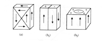
Figure 3.12. Schematic domain structures for (a ) cubic and (b) uniaxial anisotropy. The arrows show the magnetization direction.
Figure 3.13. Rux closure in ring-shaped magnets: (a ) an open circuit and (b) a closed circuit.
Let us admit the Bloch wall exists, but neglect the magnetostatic self-energy of the wall14 and assume that the material is homogeneous. Using (3.58) and (3.59) and minimizing \(E_{\text{ex}} + E_{\text{a}}\) for a wall lying in the \(y\)-\(z\)-plane (figure 3.14) then yields the Euler equations \(\phi = \pi/2\) and
\(A\frac{\partial^{2}\theta}{\partial x^{2}} - K_{1} \sin\theta \cos\theta - 2K_{2} \sin^{3}\theta \cos\theta = 0\). (3.62)
This equation has to be solved subject to the boundary condition \(\theta = 0\) and \(\theta = \pi\) for \(x = \pm\infty\), respectively. Multiplying (3.62) by \(\partial\theta/\partial x\) and integrating from \(x = -\infty\) to \(x = +\infty\) yields the implicit solution
\(x(\theta) = \sqrt{2A} \int_{0}^{\theta} \frac{1}{\sqrt{K_{1} \sin^{2}\xi + K_{2} \sin^{4}\xi}} \text{d}\xi\). (3.63)
If \(K_{2} = 0\), this reduces to the domain-wall equation
\(\theta(x) = 2 \arctan(\exp(x\sqrt{K_{1}/A}))\) (3.64)
and, since \(M_{z} = M_{\text{s}} \cos\theta\),
\(M_{z}(x) = -M_{\text{s}} \tanh(x\sqrt{K_{1}/A})\). (3.65)
14 This assumption is exact in infinite crystals but leads to corrections near surfaces.
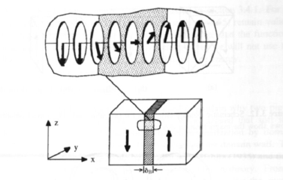
Figure 3.14. Bloch wall (schematic). \(\delta_{\text{B}}\) is the domain-wall width.
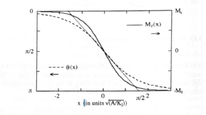
Figure 3.15. Domain-wall profiles for \(K_{1} = 0\). The dotted line refers to the commonly used definition of the wall width \(\delta_{\text{B}}\).
Figure 3.15 shows the difference between (3.64) and (3.65). For \(K_{2} > 0\) and \(K_{2} < 0\) the wall energies per unit area are
\(\gamma = 2\sqrt{AK_{2}} \left(\sqrt{\frac{K_{1}}{K_{2}}} + \frac{K_{1} + K_{2}}{K_{2}} \arcsin\sqrt{\frac{K_{2}}{K_{1} + K_{2}}}\right)\) (3.66a)
and
\(\gamma = 2\sqrt{-AK_{2}} \left(\sqrt{\frac{-K_{1}}{K_{2}}} - \frac{K_{1} + K_{2}}{K_{2}} \text{arcsinh}\sqrt{\frac{-K_{2}}{K_{1} + K_{2}}}\right)\) (3.66b)
respectively. However, in most cases it is sufficient to ignore \(K_{2}\) and use the expression
\(\gamma = 4\sqrt{AK_{1}}\). (3.66c)
Equations (3.64) and (3.65) give rise to two different definitions of the domain-wall width (figure 3.15). Most commonly one considers the function \(\theta(x)\) and uses the tangent relation \((\partial\theta/\partial x)|_{0}\delta_{\text{B}} = \pi\). This yields
\(\delta_{\text{B}} = \pi\sqrt{\frac{A}{K_{1}}}\). (3.67)
The second definition is based on the function \(M_{z}(x)\), that is the full curve in figure 3.15. Putting \((\partial M_{z}/\partial x)|_{0}\delta' = 2M_{\text{s}}\), one obtains the wall width
\(\delta' = 2\sqrt{\frac{A}{K_{1}}}\). (3.68)
The different domain wall width definitions are illustrated in figure 3.15. Typical \(\delta_{\text{B}}\) values are 50 nm and 4 nm for iron and Nd2Fe14B, respectively, whereas wall energies are of the order of 10 mJ m-2. Including \(K_{2}\), (3.67) becomes
\(\delta_{\text{B}} = \pi\sqrt{\frac{A}{K_{1} + K_{2}}}\). (3.69)
Note that there are other several types of domain wall. On the one hand, one distinguishes, for example, between 180° walls in uniaxial materials and 90° walls in cubic magnets with \(K_{1}^{u} > 0\) (figure 3.12). On the other hand, the angle \(\phi_{0}\) gives rise to a distinction between Bloch walls (\(\phi_{0} = \pi/2\)) and Néel walls (\(\phi_{0} = 0\)). Bloch walls, figure 3.14, are magnetostatically favourable in the bulk, whereas Néel walls are encountered in thin films where the absence of surface poles is important.
Single-domain Particles
Since the creation of domain walls costs energy, there are no walls if the gain in magnetostatic energy is smaller than the wall energy cost. Consider, for example, the domain configurations shown in figure 3.16. The wall energy of the two-domain configuration is \(\gamma\pi R^{2}\), whereas the gain in magnetostatic energy may be estimated as half the single-domain energy, that is \(\mu_{0}M_{\text{s}}^{2}V/12\). Since the volume of the sphere equals \(4\pi R^{3}/3\), domain formation is favourable for spheres whose radius is larger than the critical single-domain radius
\(R_{\text{sd}} = \frac{36\sqrt{AK_{1}}}{\mu_{0}M_{\text{s}}^{2}}\). (3.70)
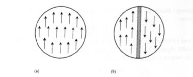
Figure 3.16. Domain formation in a sphere: (a) single-domain particle and (b) two-domain particle (schematic).
Table 3.8. Micromagnetic parameters at room temperature. The properties of Fe and Ni are uniaxial estimates (1 pJ m-1 = 10-12 J m-1).
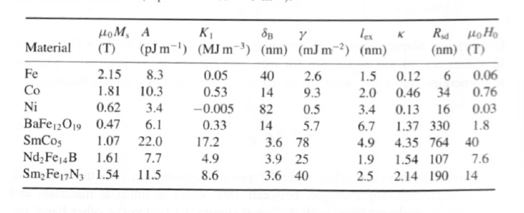
\(R_{\text{sd}}\) is of order \(0.2 \mu\)m in modern permanent magnets (table 3.8), so that any magnetic particles larger than about \(1 \mu\)m are multidomain in the ground state. Note, however, that permanent magnetism is a non-equilibrium phenomenon and it is not uncommon that reversal in single-domain particles is non-uniform (incoherent) (sections 3.2.4.2 and 3.3.3) or that the remanent state of multi-domain particles is free of domains (section 3.3.2).
Micromagnetic Scaling
By dimensional arguments, the parameters \(A\), \(K_{1}\) and \(M_{\text{s}}\) can be defined from two fundamental lengths. First, there is the exchange length
\(l_{\text{ex}} = \sqrt{\frac{A}{\mu_{0}M_{\text{s}}^{2}}}\). (3.71)
which is of the order of 3 nm for typical permanent magnets. Second, there is a wall-width parameter
\(\delta_{0} = \sqrt{A/K_{1}}\). (3.72)
We introduced the magnetic hardness parameter (1.24) \(\kappa = l_{\text{ex}}/\delta_{0}\) or
\(\kappa = \sqrt{\frac{K_{1}}{\mu_{0}M_{\text{s}}^{2}}}\). (3.73)
Magnetically very hard and very soft materials are characterized by \(\kappa \gg 1\) and \(\kappa \ll 1\), respectively. The minimum requirement for a true permanent magnet is \(H_{\text{c}} > M_{\text{s}}/2\), which implies that \(\kappa > 1/2\). In practice the coercivity is inevitably much less than the anisotropy field \(2K_{1}/\mu_{0}M_{\text{s}}\), so a better criterion for a hard magnetic material is \(M_{\text{s}} > M_{\text{s}}/2\).
The exchange length \(l_{\text{ex}}\) is the length below which atomic exchange interactions dominate typical magnetostatic fields. For example, in the next subsection we will see that \(l_{\text{ex}}\) determines the coherence radius \(R_{\text{coh}}\) below which inter-atomic exchange is able to ensure coherent rotation. It is important to note that \(l_{\text{ex}}\) is independent of \(K_{1}\) and is unrelated to the critical single-domain radius \(R_{\text{sd}}\). Another meaning of \(l_{\text{ex}}\) is that the hysteresis loop of two-phase magnets consisting of hard and soft phases is a superposition of the two individual loops if the grain size is much larger than the exchange length15.
Let us now summarize some of the previous subsections in terms of \(l_{\text{ex}}\) and \(\kappa\). The critical single-domain radius is given by
\(R_{\text{sd}} = 36\kappa l_{\text{ex}}\). (3.74)
whereas the domain-wall width is given by
\(\delta_{\text{B}} = \pi \frac{l_{\text{ex}}}{\kappa}\). (3.75)
Typical parameter values are shown in table 3.8, where we see that hard magnets are characterized by a large critical single-domain radius \(R_{\text{sd}}\) but small values of \(l_{\text{ex}}\) and \(\delta_{\text{B}}\).
Coherent Rotation: Mechanisms of Uniform Magnetization Reversal
Up until now we have been considering domain structures, which amounts to a search for global energy minima. In fact, hysteresis is caused by metastable local energy minima (figure 3.1). A very simple hysteresis mechanism is coherent rotation, where the term coherent means that the magnetization remains uniform throughout the magnet. Although coherent rotation is not very common in real
materials, it reproduces many of the features in an easy-to-follow way. From a formal point of view, coherent rotation is obtained by setting \(\nabla(M/M_{\text{s}}) = 0\) in (3.53). Let us for the moment consider isotropic magnets, whose self-interaction energy does not depend on the magnetization direction. Then
\(E_{\text{s}} = \int [K_{1} \sin^{2}\theta + K_{2} \sin^{4}\theta - \mu_{0}M_{\text{s}}H \cos(\Theta - \theta)] \text{d}V\) (3.76)
where \(\Theta\) is the angle between the \(z\)-axis and the field direction.
Zero-field Spin Configurations
Putting \(H = 0\) in (3.76) yields a number of energy landscapes (figure 3.17). A particularly interesting regime is the easy-cone magnetism occurring if the conditions \(K_{1} < 0\) and \(K_{2} > -K_{1}/2\) are satisfied simultaneously. The tilt angle between the \(z\)-axis and the easy magnetization direction is given by
\(\theta_{\text{c}} = \arcsin\sqrt{\frac{|K_{1}|}{2K_{2}}}\). (3.77)
Permanent magnets are characterized by easy-axis magnetism, but it is not uncommon that the more pronounced temperature dependence of \(K_{2}\) yields a spin reorientation transition from easy-axis to easy-plane or easy-cone magnetism at low temperatures. Examples are ErFe14B, which exhibits easy-plane anisotropy below \(T_{\text{sr}} = 325\) K but easy-axis anisotropy above \(T_{\text{sr}}\), and Nd2Fe14B, which is easy axis at room temperature but easy cone below the spin-tilt temperature \(T_{\text{st}} = 135\) K (section 5.3.2.1).
Anisotropy Fields
In section 3.1.1.4 we emphasized that \(H_{0} = 2K_{1}/\mu_{0}M_{\text{s}}\) is not the only anisotropy-field definition. Consider an easy-axis magnet in a perpendicular field \(H = He_{x}\). Taking into account the fact that \(\Theta = \pi/2\) and \(M_{x} = M_{\text{s}} \sin\theta\) and minimizing the energy with respect to \(M_{x}\) yields
\(H = \frac{2K_{1}}{\mu_{0}M_{\text{s}}} \frac{M_{x}}{M_{\text{s}}} + \frac{4K_{2}}{\mu_{0}M_{\text{s}}} \frac{M_{x}^{3}}{M_{\text{s}}^{3}}\). (3.78)
To achieve saturation, that is \(M_{x} = M_{\text{s}}\), one has to apply the anisotropy field
\(H_{\text{k}}' = \frac{2K_{1} + 4K_{2}}{\mu_{0}M_{\text{s}}}\). (3.79)
A third anisotropy-field definition, namely
\(H_{\text{a}} = \frac{2K_{1} + 2K_{2}}{\mu_{0}M_{\text{s}}}\) (3.80)
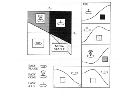
Figure 3.17. The magnetic phase diagram for uniaxial magnets.
is obtained from (3.76) by setting \(H = 0\) and analysing the energy difference \(E(\pi/2) - E(0)\). This means that it is not possible to define an anisotropy field which incorporates \(K_{1}\) and \(K_{2}\) in a universal way.
From (3.78) we see that plotting \(H/M_{x}\) versus \(M_{x}^{2}\) makes it possible to deduce \(K_{1}\) and \(K_{2}\) from experimental data. This procedure is known as the Sucksmith–Thompson method. However, small deviations from \(\Theta = 90^{\circ}\) are sufficient to suppress alignment \((M_{x} = M_{\text{s}})\) in any finite field, so that caution must be exercised when applying the method to imperfectly aligned magnets.
Angular Dependence
In the context of hysteresis loops, the coherent-rotation mechanism is known as the Stoner–Wohlfarth model (1948). If the magnetic field and the easy-axis direction are parallel, that is for \(H = 0\), the hysteresis loop deduced from (3.76) is rectangular and the coercivity equals the anisotropy field \(H_{0} = 2K_{1}/\mu_{0}M_{\text{s}}\). Non-zero angles \(\Theta\) describe, for example, ensembles of misaligned magnetic particles (section 3.3.5.1). This refers not only to isotropic magnets but also to partly aligned or textured magnets, where the easy-axis distribution is described by a function \(P(\Theta)\). Essentially, the energy expression (figure 3.18) shows the magnetic energy for \(K_{2} = 0\) and a grain misalignment of \(\Theta = 30^{\circ}\). Small reverse fields, \(|H| < H_{0}\), yield a reversible rotation of the magnetization direction, but in large reverse fields the metastable energy minimum \((M_{x} > 0)\)
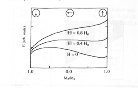
Figure 3.18. The magnetization dependence of the magnetic energy (\(\Theta = 30^{\circ}\)).
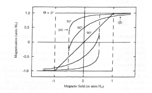
Figure 3.19. The dependence of the magnetization on the angle \(\Theta\) between field and easy axis. Dashed lines indicate magnetization jumps. The meaning of the symbols \((\alpha)\) and \((\beta)\) is explained in the text.
vanishes and the magnetization switches irreversibly into the global minimum \((M_{z} < 0)\).
Plotting \(M_{z}\) as a function of the external field yields the hysteresis loops of figure 3.19. With increasing misalignment angle the loops narrow and at \(\Theta = 90^{\circ}\), when the field is perpendicular to the easy axis, hysteresis vanishes completely. The symbol \((\alpha)\) indicates the instability of the metastable energy minimum shown in figure 3.18. Finite fields do not lead to saturation in the intermediate regime \(0 < \Theta < \pi/2\), where the approach to saturation obeys a \(1/H^{2}\) power law. In figure 3.19, one of these branches is denoted by \((\beta)\). The angular dependence of the hysteresis loops should not be confused with the
phenomenon of rotational hysteresis caused by revolving the external magnetic field.
The Stoner–Wohlfarth theory applies fairly well to weakly interacting ensembles of nanoparticles. We will discuss this important aspect in the context of nanostructured permanent magnets (section 3.3.5).
Magnetostatic Interaction and Shape Anisotropy
In their 1948 paper, Stoner and Wohlfarth assumed that \(K_{1}\) is dominated by shape anisotropy (section 3.1.2.1). In fact, shape anisotropy is important in semihard materials such as alnico and CrO2, and it is in order now to elaborate the relation between coherent rotation and shape anisotropy.
The starting point is the magnetostatic self-interaction energy \(E_{\text{dm}} = -(\mu_{0}/2) \int M \cdot H_{\text{dm}} \text{d}V\). Using (2.66) we obtain
\(E_{\text{dm}} = \frac{\mu_{0}}{2} (D_{\perp}M_{x}^{2} + D_{\perp}M_{y}^{2} + D_{\parallel}M_{z}^{2})V\) (3.81)
and, with (3.1),
\(E_{\text{dm}} = \frac{\mu_{0}}{2} M_{\text{s}}^{2}V(D_{\perp} \sin^{2}\theta + D_{\parallel} \cos^{2}\theta)\). (3.82)
Now \(2D_{\perp} + D_{\parallel} = 1\) and \(\sin^{2}\theta + \cos^{2}\theta = 1\) yield
\(E_{\text{der}} = \frac{\mu_{0}}{2} D_{\parallel}M_{\text{s}}^{2}V + \frac{\mu_{0}}{4} M_{\text{s}}^{2}V(1 - 3D_{\parallel})\sin^{2}\theta\). (3.83)
In this equation, the \(\theta\)-independent term amounts to a physically irrelevant shift of the zero-point energy, whereas the \(\sin^{2}\theta\) term yields the shape anisotropy (3.8) we are seeking.
Equation (3.83) predicts an easy-axis shape-anisotropy contribution for prolate ellipsoids, where \(D_{\parallel} = D < 1/3\). On the other hand, there is no shape anisotropy in spherical magnets (\(D = 1/3\)). The absence of shape anisotropy in spheres means that the magnetostatic energy of a uniformly magnetized sphere is independent of the magnetization direction. This example shows that shape anisotropy is only indirectly related to the demagnetizing field \(-DM\), which never gives rise to an easy-axis-type contribution. As mentioned in the context of figure 3.11, the reason for this counterintuitive disagreement is that the incoherent nucleation modes violate the assumption of coherent rotation (section 3.2.4.3).
Nucleation in Homogeneous Ellipsoids: Insights into Magnetic Reversal
Consider a magnet which has been magnetized in a strong magnetic field, so that the magnetization is captured in a generally metastable energy minimum. Nucleation is then defined as an instability of this minimum in a reverse field. For example, figures 3.18 and 3.19 show that grains misaligned
by 30° exhibit a nucleation instability at the nucleation field \(H_{\text{N}} = H_{0}/2\). In terms of the local magnetization \(M(\mathbf{r})\), nucleation processes are realized by nucleation modes. The idea is to restrict the consideration to the immediate vicinity of the nucleation field \(\mathbf{H} = -H_{\text{N}}\mathbf{e}_{z}\), where the magnetization is \(\mathbf{M}_{\text{N}}\). The equation
\(\mathbf{M}(\mathbf{r}) = M_{\text{N}}(\mathbf{r})\sqrt{1 - \mathbf{m}(\mathbf{r})^{2}} + M_{\text{s}}(\mathbf{r})\mathbf{m}(\mathbf{r})\) (3.84)
subject to \(\mathbf{m}(\mathbf{r}) \cdot \mathbf{M}_{\text{N}}(\mathbf{r}) = 0\) defines a dimensionless magnetization variable \(\mathbf{m}(\mathbf{r})^{16}\). To linearize the nucleation problem we expand \(\mathbf{M}(\mathbf{r})\) into powers of the small quantity \(\mathbf{m}(\mathbf{r})\):
\(\mathbf{M}(\mathbf{r}) = M_{\text{N}}(\mathbf{r}) \left(1 - \frac{\mathbf{m}(\mathbf{r})^{2}}{2}\right) + M_{\text{s}}(\mathbf{r})\mathbf{m}(\mathbf{r})\). (3.85)
Putting this expression into the magnetic energy functional and neglecting higher-order terms yields a quadratic expression which can be solved by eigenmode analysis, and the eigenfunction \(\mathbf{m}(\mathbf{r})\) describing the nucleation instability is the nucleation mode.
The determination of nucleation fields and modes in homogeneous ellipsoids of revolution is one of the few exactly solvable model problems in many-body physics. We will see that these nucleation modes are extended, that is \(\mathbf{m}(\mathbf{r})\) extends throughout the magnetic ellipsoid (figure 3.11). By comparison, nucleation in real magnets tends to be localized due to morphological inhomogeneities (section 3.3.3).
Stoner–Wohlfarth Model
A simple nucleation mechanism is associated with the Stoner–Wohlfarth model. Consider a homogeneous and aligned ellipsoid of revolution (\(D_{\parallel} = D\)), where both the easy axis (\(\mathbf{n}\)) and the axis of revolution are parallel to the field direction \(\mathbf{e}_{z}\). In the limit of coherent rotation we obtain from (3.76) and (3.83) the magnetic energy
\(\frac{E}{V} = K_{1} \sin^{2}\theta + \frac{\mu_{0}}{4}(1 - 3D)M_{\text{s}}^{2} \sin^{2}\theta + K_{2} \sin^{4}\theta - \mu_{0}M_{\text{s}}H \cos\theta\). (3.86)
Expanding this expression in terms of the small quantity \(\theta\) we obtain the equation
\(\frac{E}{V} = \left(K_{1} + \frac{\mu_{0}}{4}(1 - 3D)M_{\text{s}}^{2} + \frac{1}{2}\mu_{0}M_{\text{s}}H\right) \theta^{2}\) (3.87)
which is suitable for eigenmode analysis17. The nucleation field \(H_{\text{N}}\) is the reverse field at which the energy minimum (3.87) vanishes (\(\partial^{2}E/\partial\theta^{2} = 0\)).
16 The functional structure of (3.84) is given by the requirement \(M(\mathbf{r})^{2} = M_{\text{s}}(\mathbf{r})^{2}\).
17 Note that \(M_{\text{N}}(\mathbf{r}) = M_{\text{s}}\mathbf{e}_{z}\), that is \(\theta = 0\), and \(|\mathbf{m}| = \sin\theta\).
From a formal point of view, the solution
\(H_{\text{N}} = \frac{2K_{1}}{\mu_{0}M_{\text{s}}} + \frac{1}{2}(1 - 3D)M_{\text{s}}\) (3.88)
is equivalent to (1.28). However, \(H_{\text{N}}\) denotes an exact eigenvalue, whereas \(H_{\text{c}}\) in (1.26) is frequently interpreted as a coercivity estimate. The corresponding nucleation mode is the uniform or coherent-rotation mode \(\theta(\mathbf{r}) = \theta_{0}\), where \(\theta_{0} \ll \pi/2\).
There are two important points about (3.88). First, the nucleation field is independent of \(K_{2}\), because \(K_{2}\) contributions scale as \(\sin^{4}\theta \approx \theta^{4}\). Only in misaligned magnets, where \(\mathbf{n} \neq \mathbf{e}_{z}\), does there exist a non-zero \(K_{2}\) contribution to the nucleation field. Second, the field entering (3.87) is the external field \(H\); in the present context, there is no simple interpretation of the internal field \(H' = H - DM\).
Incoherent Nucleation
The strength of the exchange interaction ensures time-averaged ferromagnetic spin alignment on an atomic scale and gives rise to coherent magnetization processes in small magnets. However, on a macroscopic scale, magnetostatic interaction and magnetocrystalline anisotropy lead to deviations from the ideal spin alignment.
To introduce the problem of incoherent nucleation we consider the hemisphere model shown in figure 3.20. The moments \(m = M_{\text{s}}V/2\) of the hemispheres a and b are assumed to reside at \(\mathbf{r}_{\text{a}} = -Re_{x}/2\) and \(\mathbf{r}_{\text{b}} = +Re_{x}/2\), respectively. Furthermore, we make the intuitive assumption that the dimensionless magnetizations \(\mathbf{s}_{\text{a/b}} = 2\mathbf{m}_{\text{a/b}}/M_{\text{s}}V\) of the hemispheres lie in the \(y\)-\(z\)-plane: \(\mathbf{s}_{\text{a/b}} = e_{z} \cos\theta_{\text{a/b}} + e_{y} \sin\theta_{\text{a/b}}\). Putting \(K_{2} = 0\), \(\mathbf{H} = -He_{z}\) and \(\mathbf{n} = e_{z}\), and neglecting higher-order powers of \(\theta_{\text{a/b}}\) yields the magnetic energy
\(\frac{E}{V} = \left(\frac{A}{R^{2}} - \frac{1}{24}\mu_{0}M_{\text{s}}^{2}\right)(\theta_{\text{a}} - \theta_{\text{b}})^{2} + \frac{1}{4}(2K_{1} - \mu_{0}M_{\text{s}}H)(\theta_{\text{a}}^{2} + \theta_{\text{b}}^{2})\). (3.89)
Here the estimate \(A/R^{2}\) has been used for the average exchange-energy density. Stability analysis of (3.89), that is diagonalization of the \(2 \times 2\) matrix \(\partial^{2}E_{\text{m}}/\partial\theta_{\text{a}}\partial\theta_{\text{b}}\), yields the nucleation field \(H_{\text{N}}\). There are two eigenmodes: a coherent mode \(\theta_{\text{coh}} = \theta_{\text{a}} + \theta_{\text{b}}\) with the familiar Stoner–Wohlfarth nucleation field \(2K_{1}/\mu_{0}M_{\text{s}}\), and an incoherent mode \(\theta_{\text{incoh}} = \theta_{\text{a}} - \theta_{\text{b}}\) where
\(H_{\text{N}} = \frac{2K_{1}}{\mu_{0}M_{\text{s}}} - \frac{1}{3}M_{\text{s}} + \frac{8A}{\mu_{0}M_{\text{s}}R^{2}}\). (3.90)
The geometrical meaning of these two modes is illustrated in figure 3.20.
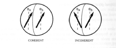
Figure 3.20. Coherent and incoherent nucleation ( schematic ).
Comparing the two nucleation fields, we find that incoherent nucleation is favourable in particles whose radius is larger than the coherence radius
\(R_{\text{coh}} = \sqrt{\frac{24A}{\mu_{0}M_{\text{s}}^{2}}}\). (3.91)
This coherence radius, about \(5l_{\text{ex}}\), is of the order of 10 nm for typical permanent magnets (table 3.8). The physics behind this result is that the incoherent mode in figure 3.20 is magnetostatically favourable, because the hemisphere moments exhibit an antiparallel component. This gain in magnetostatic energy has to compete against the exchange energy but dominates in large particles. Note that \(K_{1}\) does not enter (3.91), because both coherent and incoherent rotation exhibit the same \(K_{1}\) contribution to the nucleation field. From (3.71) and (3.74) we see that \(R_{\text{coh}}\) must not be confused with the critical single-domain particle radius \(R_{\text{sd}}\). In true permanent magnets, \(R_{\text{sd}} \gg R_{\text{coh}}\).
Magnetization Curling
The main difference between the hemispheres, figure 3.20, and homogeneous ellipsoids of revolution is that the simplified model has two degrees of freedom, \(\theta_{\text{a}}\) and \(\theta_{\text{b}}\), whereas the magnetization of real particles is continuous. However, it turns out that the exact nucleation field does not differ very much from the hemisphere solution.
The curling mechanism, illustrated in figures 3.11 and 3.21, is defined by \(M_{\text{N}}(\mathbf{r}) = M_{\text{s}}\mathbf{e}_{z}\) and
\(\mathbf{m}(\mathbf{r}) = F\left(z,\sqrt{x^{2}+y^{2}}\right) \frac{x\mathbf{e}_{y} - y\mathbf{e}_{x}}{\sqrt{x^{2}+y^{2}}}\). (3.92)
Putting
\(\mathbf{M}(\mathbf{r}) = M_{\text{s}} \left(1 - \frac{\mathbf{m}(\mathbf{r})^{2}}{2}\right) \mathbf{e}_{z} + M_{\text{s}}\mathbf{m}(\mathbf{r})\) (3.93)
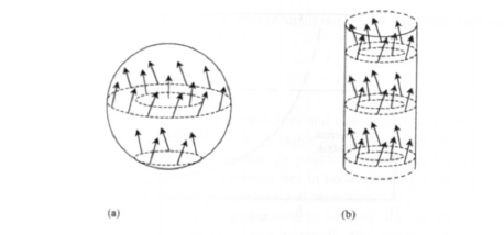
Figure 3.21. The curling nuclcation mode in (a) spheres and (b) infinite cylinders. The arrows show the magnetization.
into the energy functional (3.52) and expanding the result with respect to the small transverse magnetization component \(M_{\text{s}}\mathbf{m}(\mathbf{r})\) one obtains, after some calculation,
\(E = \int \left(A(\nabla\mathbf{m})^{2} + \left[K_{1} + \frac{1}{2}\mu_{0}M_{\text{s}}(H - DM_{\text{s}})\right] \mathbf{m}^{2}\right) \text{d}V\). (3.94)
It is important to note that the demagnetizing-field term in this equation originates from the \(z\)-component of the magnetization (3.93). The transverse field component does not contribute to the magnetostatic self-energy, because it forms closed flux lines.
Minimizing this equation with respect to \(\mathbf{m}(\mathbf{r})\) yields the differential equation
\(-2A\nabla^{2}\mathbf{m} + (2K_{1} + \mu_{0}M_{\text{s}}(H - DM_{\text{s}}))\mathbf{m} = 0\) (3.95)
subject to the boundary condition \(\mathbf{e}_{\text{s}} \cdot \nabla\mathbf{m} = 0\), where \(\mathbf{e}_{\text{s}}\) is the surface normal.
The ansatz (3.92) transforms (3.95) into a differential equation for \(F\) whose solution yields the curling mode we are seeking18. The nucleation field is given by
\(H_{\text{N}} = \frac{2K_{1}}{\mu_{0}M_{\text{s}}} - DM_{\text{s}} + \frac{cA}{\mu_{0}M_{\text{s}}R^{2}}\) (3.96a)
where \(c = 8.666\) for spheres (\(D = 1/3\)) and \(c = 6.678\) for needles (\(D = 0\)). The radius \(R = R_{x} = R_{y}\) refers to the two degenerate axes of the ellipsoid. As in the case of coherent rotation, this equation applies to both zero and non-zero anisotropy constants \(K_{2}\).
It is important to note that (3.96) is an exact result, because the curling mode is an eigenfunction of the differential equation (3.95). By contrast, calculated
18 For infinite cylinders (\(D = 0\)) and spheres (\(D = 1/3\)) the solutions are the ordinary and spherical Bessel functions \(J_{1}\) and \(j_{1}\), respectively. For other shapes see Aharoni (1966).
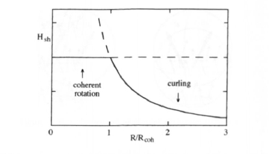
Figure 3.22. The shape-anisotropy contribution to the nucleation field of a prolate ellipsoid. For coherent rotation, \(\Delta H_{\text{N}} = (1 - D)M_{\text{s}}/2\).
critical single-domain radii are approximate, because they depend on the choice of the domain-wall geometry. Comparing (3.90) and (3.96) we see that the hemisphere nucleation field does not differ very much from the exact solution.
The 'intrinsic' coercivity \(H_{\text{c}}\) used in practice (section 3.3.1.1) refers to a closed circuit (\(D = 0\)), so that we have to subtract the demagnetizing field \(-DM_{\text{s}}\) from (3.88) and (3.96). Assuming that the coercivity is determined by \(H_{\text{N}}\) we then obtain for coherent rotation and curling the respective expressions
\(H_{\text{c}} = \frac{2K_{1}}{\mu_{0}M_{\text{s}}} + \frac{1}{2}(1 - D)M_{\text{s}}\) (3.88b)
and
\(H_{\text{c}} = \frac{2K_{1}}{\mu_{0}M_{\text{s}}} + \frac{c(D)A}{\mu_{0}M_{\text{s}}R^{2}}\). (3.96b)
These equations can be rewritten as \(H_{\text{c}} = 2K_{0}/\mu_{0}M_{\text{s}} + H_{\text{sh}}\), where \(H_{\text{sh}}\) is the shape-anisotropy contribution to the intrinsic coercivity (figure 3.22). Equation (3.96b) shows that there is no shape-anisotropy contribution to the intrinsic coercivity of macroscopic magnets. On the other hand, in finite-size magnets the subtraction of the demagnetizing field is not able to remove the shape dependence of the coercivity. In fact, since \(c(D)\) depends on the sample shape, there is an interference between magnetostatic demagnetization and exchange interactions (figure 3.11). In section 3.3.1.2 we will see how this affects the interpretation of hysteresis loops.
Coherent rotation and curling are the only nucleation modes in oblate ellipsoids, spheres and moderately elongated prolate ellipsoids. For ellipsoids whose lengths exceed 9.2 times the radii, a third mode, namely buckling, cannot be ruled out for \(R < 4l_{\text{ex}}\). Buckling is a sinoidal modulation of the magnetization in the \(z\)-direction whose period (wavelength) depends on the ratio \(R/l_{\text{ex}}\). Since the period is at least about ten times larger than the radius, buckling and coherent rotation are very similar, and in the limit of small radii R the buckling mechanism degenerates into coherent rotation.


